
Chapter 5. Texture Mapping
Texture mapping is the process of adding detail to the surface of a 3D object. This can be likened to gift wrapping, where your wrapping paper is a 2D texture. Texture mapping is fundamental to modern rendering and is used for a multitude of interesting graphics techniques.
An Introduction to Texture Mapping
Generally, you’ll want more detail in your rendered 3D objects than the solid color produced by the HelloShader and HelloStructs effects from the last chapter. As you’ve learned, 3D models consist of vertices, typically organized into triangles. Those vertices are described, at a minimum, by a position. But they can contain additional information. A step toward additional surface detail is to provide a color for each vertex. Consider the 3D cubes in Figure 5.1.
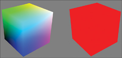
On the cube to the left, each vertex is supplied a different color; on the right, each vertex has the same color. Clearly, the cube on the left has more detail. The colors add interest to the object and help define the faces of the cube. Furthermore, the colors of the individual pixels vary with respect to their positions relative to the vertices (recall the discussion of interpolation during the rasterizer stage from Chapter 1, “Introducing DirectX”). You gain more control over the color of a surface by increasing the number of colored vertices that make up your 3D objects. However, when viewed close up, you’ll never have enough vertices to produce a high-quality rendering, and any such attempt would quickly yield an overwhelming number of vertices. The solution is texture mapping.
To map a texture to a triangle, you include two-dimensional coordinates with each vertex. You use those coordinates to look up a color stored in a 2D texture. And you do this lookup in the pixel shader to find the color for each pixel of the triangle. The texture coordinates, then, are interpolated from the triangle vertices instead of the vertex color.
DirectX texture coordinates range from 0 to 1 (inclusive) on both the horizontal and vertical axes, where the origin is the top-left corner. These axes are commonly given the names u (horizontal) and v (vertical). Figure 5.2 shows a texture mapped to a quad (two triangles) and highlights the texture coordinates for each vertex.
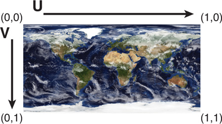
Figure 5.2 DirectX 2D texture coordinates. (Original texture from Reto Stöckli, NASA Earth Observatory. Additional texturing by Nick Zuccarello, Florida Interactive Entertainment Academy.)
Note
Direct3D supports 1D, 2D, and 3D textures along with texture arrays and texture cubes (discussed further in Chapter 8, “Gleaming the Cube”). The number of coordinates required for lookup matches the dimensionality of the texture.
A Texture Mapping Effect
Listing 5.1 presents the code for a texture mapping effect. As before, create a new effect/material in NVIDIA FX Composer and transpose the code from the listing. Then you can examine this code step by step.
/************* Resources *************/
#define FLIP_TEXTURE_Y 1
cbuffer CBufferPerObject
{
float4x4 WorldViewProjection : WORLDVIEWPROJECTION < string
UIWidget="None"; >;
}
RasterizerState DisableCulling
{
CullMode = NONE;
};
Texture2D ColorTexture <
string ResourceName = "default_color.dds";
string UIName = "Color Texture";
string ResourceType = "2D";
>;
SamplerState ColorSampler
{
Filter = MIN_MAG_MIP_LINEAR;
AddressU = WRAP;
AddressV = WRAP;
};
/************* Data Structures *************/
struct VS_INPUT
{
float4 ObjectPosition : POSITION;
float2 TextureCoordinate : TEXCOORD;
};
struct VS_OUTPUT
{
float4 Position : SV_Position;
float2 TextureCoordinate : TEXCOORD;
};
/************* Utility Functions *************/
float2 get_corrected_texture_coordinate(float2 textureCoordinate)
{
#if FLIP_TEXTURE_Y
return float2(textureCoordinate.x, 1.0 - textureCoordinate.y);
#else
return textureCoordinate;
#endif
}
/************* Vertex Shader *************/
VS_OUTPUT vertex_shader(VS_INPUT IN)
{
VS_OUTPUT OUT = (VS_OUTPUT)0;
OUT.Position = mul(IN.ObjectPosition, WorldViewProjection);
OUT.TextureCoordinate = get_corrected_texture_coordinate(IN.
TextureCoordinate);
return OUT;
}
/************* Pixel Shader *************/
float4 pixel_shader(VS_OUTPUT IN) : SV_Target
{
return ColorTexture.Sample(ColorSampler, IN.TextureCoordinate);
}
/************* Techniques *************/
technique10 main10
{
pass p0
{
SetVertexShader(CompileShader(vs_4_0, vertex_shader()));
SetGeometryShader(NULL);
SetPixelShader(CompileShader(ps_4_0, pixel_shader()));
SetRasterizerState(DisableCulling);
}
}
Comments, the Preprocessor, and Annotations
A number of language constructs come into play from this effect. First, notice the comments organizing the effect. HLSL supports C++-style single-line comments (// comments) and multiline comments (/* comments */).
Next, recognize the #define FLIP_TEXTURE_Y 1 macro at the top of the effect. This has behavior identical to the C/C++ #define directive. Indeed, HLSL has several familiar preprocessor commands, including #if, #else, #endif, and #include.
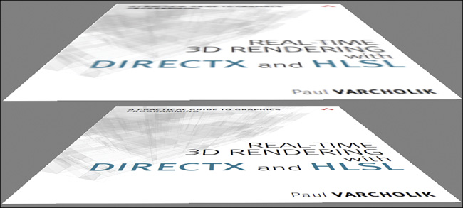
Now examine the WorldViewProjection shader constant, declared within the cbuffer. This constant has the same behavior as in HelloShaders and HelloStructs, but you’ve added an annotation to the end of the declaration. Annotations are notes to the CPU-side application and are enclosed in angled brackets. These notes do not affect shader execution, but the application can use them. For example, the UIWidget annotation, attached to WorldViewProjection, controls how NVIDIA FX Composer treats that shader constant. With a value of None, NVIDIA FX Composer hides the shader constant from the list of visible material properties. Figure 5.3 shows the NVIDIA FX Composer Properties panel both without the annotation (left) and with the annotation to hide the constant (right). Note that this only hides the value from the Properties panel; the CPU still updates the constant. Hiding the constant makes sense for the WorldViewProjection matrix because you won’t be hand-editing that matrix.
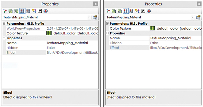
Figure 5.3 NVIDIA FX Composer Properties panel showing the properties for TextureMapping.fx without the UIWidget="None" annotation on WorldViewProjection (left) and with the annotation (right).
Texture Objects and Samplers
Three steps are involved in using a texture within an HLSL effect. First, you must declare the texture object (see Listing 5.2). An HLSL texture declaration can use the explicit subtype (such as Texture2D) or the more generic texture data type. Texture objects cannot be declared within cbuffers.
Listing 5.2 The Texture Object Declaration from TextureMapping.fx
Texture2D ColorTexture <
string ResourceName = "default_color.dds";
string UIName = "Color Texture";
string ResourceType = "2D";
>;
Three annotations are associated with the ColorTexture variable in Listing 5.2. As with all annotations, these are optional, but in the context of NVIDIA FX Composer, these annotations offer enhanced usability.
The UIName annotation enables you to customize the displayed variable name within the Properties panel. ResourceType identifies the type of texture that can be assigned, and ResourceName allows a default texture to be used when the user has not supplied one.
Next, you must declare and initialize a texture sampler (see Listing 5.3). Samplers control how a color is retrieved from a texture. Direct3D 10 introduced the SamplerState data type, and it directly maps to a corresponding Direct3D C struct with members for filtering and texture address modes. We discuss these topics shortly.
Listing 5.3 The Sampler Object Declaration from TexureMapping.fx
SamplerState ColorSampler
{
Filter = MIN_MAG_MIP_LINEAR;
AddressU = WRAP;
AddressV = WRAP;
};
The final step is to sample the texture using the declared sampler object. This step is performed in the pixel shader (see Listing 5.4).
Listing 5.4 The Pixel Shader from TextureMapping.fx
float4 pixel_shader(VS_OUTPUT IN) : SV_Target
{
return ColorTexture.Sample(ColorSampler, IN.TextureCoordinate);
}
Note the C++-style method invocation of the Sample() method against the ColorTexture object. The first argument to the Sample() method is the sampler object, followed by the coordinates to look up in the texture.
Texture Coordinates
The vertex stream supplies the coordinates for sampling the texture, with corresponding members in the VS_INPUT and VS_OUTPUT data structures (see Listing 5.5). Observe the TEXCOORD semantics attached to the 2D TextureCoordinate members.
Listing 5.5 The Vertex Shader Input and Output Data Structures from TextureMapping.fx
struct VS_INPUT
{
float4 ObjectPosition : POSITION;
float2 TextureCoordinate : TEXCOORD;
};
struct VS_OUTPUT
{
float4 Position : SV_Position;
float2 TextureCoordinate : TEXCOORD;
};
The vertex shader (see Listing 5.6) passes the input texture coordinates to the output of the stage, but it does so after invoking get_corrected_texture_coordinate(). HLSL supports user-defined, C-style helper functions, and this one simply inverts the vertical texture coordinate if FLIP_TEXTURE_Y is nonzero. This is necessary within NVIDIA FX Composer because it uses OpenGL-style texture coordinates for the built-in 3D models (the Sphere, Teapot, Torus, and Plane). The origin for OpenGL texture coordinates is the bottom-left corner instead of the top-left corner for DirectX. Therefore, when you’re visualizing your shaders in NVIDIA FX Composer against one of the built-in models, you need to flip the vertical texture coordinate. If you import a custom model into NVIDIA FX Composer and that model has DirectX-style texture coordinates, you can disable the FLIP_TEXTURE_Y macro.
Listing 5.6 The Vertex Shader and a Utility Function from TextureMapping.fx
float2 get_corrected_texture_coordinate(float2 textureCoordinate)
{
#if FLIP_TEXTURE_Y
return float2(textureCoordinate.x, 1.0 - textureCoordinate.y);
#else
return textureCoordinate;
#endif
}
VS_OUTPUT vertex_shader(VS_INPUT IN)
{
VS_OUTPUT OUT = (VS_OUTPUT)0;
OUT.Position = mul(IN.ObjectPosition, WorldViewProjection);
OUT.TextureCoordinate = get_corrected_texture_coordinate(IN.
TextureCoordinate);
return OUT;
}
Texture Mapping Output
Figure 5.4 shows the output of the texture mapping effect applied to a sphere with a texture of Earth.
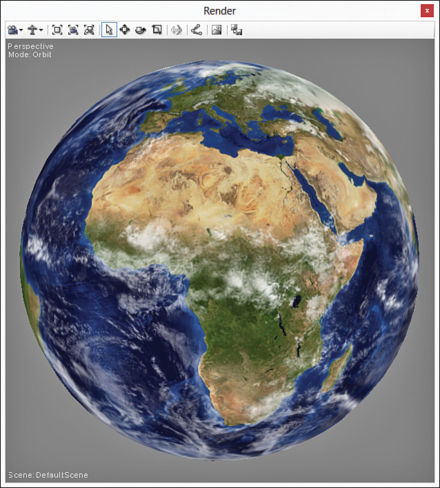
Figure 5.4 TextureMapping.fx applied to a sphere with a texture of Earth. (Original texture from Reto Stöckli, NASA Earth Observatory. Additional texturing by Nick Zuccarello, Florida Interactive Entertainment Academy.)
Texture Filtering
In our discussion of texture coordinates and sampling, you might have realized that you will rarely view a texture-mapped object at a one-to-one correspondence between the elements in the texture (texels) and the pixels rendered to the screen. Your camera will be at an arbitrary distance from the textured object and will view it at an arbitrary angle. Consider a scenario in which the camera is “zoomed in” to a textured object. The rasterizer stage determines which pixels to send to the pixel shader and interpolates their texture coordinates. But the coordinates represent locations that are in between authored texels in the texture. In other words, you’re trying to render the texture at a higher resolution than it was authored. The topic of texture filtering determines what color should be chosen for these pixels because they have no direct lookup in the texture.
Magnification
The scenario just described is known as magnification—in this situation, there are more pixels to render than there are texels. Direct3D supports three types of filtering to determine the colors of these “in between” pixels: point filtering, linear interpolation, and anisotropic filtering.
Point Filtering
Point filtering is the fastest of the filtering options, but it generally yields the lowest quality results. Also known as nearest-neighbor filtering, point filtering simply uses the color of the texel closest to the pixel center. Shown on the left side of Figure 5.5, you can see the blocky-looking image produced with point filtering.
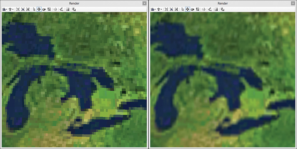
Figure 5.5 The results of point filtering (left) and bilinear interpolation (right) on a magnified texture. (Texture by Reto Stöckli, NASA Earth Observatory.)
Linear Interpolation
A higher-quality filtering option is linear interpolation, in which the color is interpolated between neighboring texels. For 2D textures, this is more correctly named bilinear interpolation because the interpolation takes place both horizontally and vertically. In this filtering technique, the four texels surrounding the pixel center are identified and two 1D linear interpolations are performed for the pixels along the u-axis. Then a third interpolation is performed along the v-axis to produce the final color. The image on the right side of Figure 5.5 shows the same magnified texture using bilinear interpolation. Notice the smoother appearance of this image compared to point filtering.
Anisotropic Filtering
Anistropy refers to the distortion of a texture projected onto a surface that is at an oblique angle to the camera. Anisotropic filtering reduces this distortion and improves the rendered output. This is the most expensive filtering option, but the results are compelling. Figure 5.6 compares a texture mapped object with and without anisotropic filtering.
Minification
Minification is the opposite of magnification and applies when a pixel covers more than one texel. This happens as the camera gets farther from a textured surface and Direct3D must choose the appropriate color. The same filtering options apply, but it’s a bit more complicated for minification. With linear interpolation, for example, the four texels surrounding the pixel center are identified just as they were for magnification. However, the in-between texels (the multiple colors occupying the same lookup for the pixel center) are ignored and don’t contribute to the final color. This can produce artifacts that decrease rendering quality.
You might envision an approach in which the texels are averaged to produce a better result. However, such computation is based on the resolution of the down-sampled texture, and an arbitrary number of “levels” can be computed. Building these levels on the fly would be impractical. Instead, this approach can be precomputed through a technique known as mipmapping.
Mipmaps
Mipmaps are smaller versions of the original texture, typically precomputed and stored within the same file. Each mip-level is a progressive division by 2, down to a 1×1 texture. Figure 5.7 shows an example of the Earth texture at a size of 512×256 with nine mip-levels.
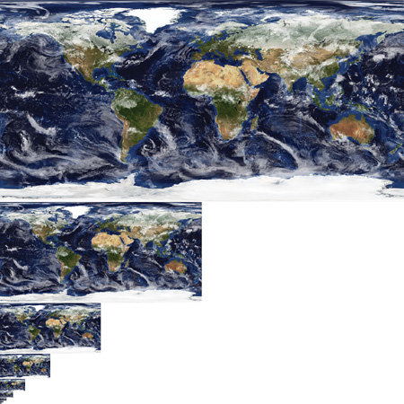
Figure 5.7 A mipmapped Earth texture with nine mip-levels. (Original texture from Reto Stöckli, NASA Earth Observatory. Additional texturing by Nick Zuccarello, Florida Interactive Entertainment Academy.)
When employing mipmaps, two steps are required to produce a final color. First, the mip-level (or levels) must be selected for minification or magnification. Second, the selected mip-level(s) is filtered to derive a color.
Point or linear filtering can be used to select a mip-level. Point filtering simply selects the nearest mip-level, and linear filtering selects the two surrounding mipmaps. Then the selected mip-level is sampled through point, linear, or anisotropic filtering. If linear filtering was used to select the two neighboring mipmaps, both mip-levels are sampled and their results are interpolated. This technique produces the highest-quality results.
Finally, although mipmapping improves rendering quality, note that it also increases memory requirements by 33 percent.
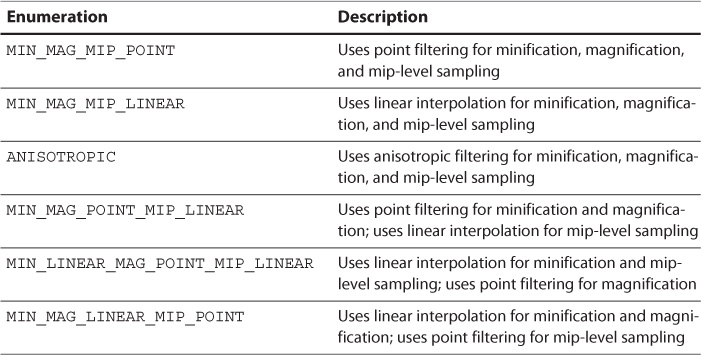
SamplerState Filtering Options
Refer to the SamplerState object from TextureMapping.fx (reproduced in Listing 5.7), and you’ll notice the Filter member and its assigned value of MIN_MAG_MIP_LINEAR. This configures the sampler to use linear interpolation for minification, magnification, and mip-level sampling. Direct3D allows independent configurations for each of these elements. Table 5.1 provides examples of the various permutations. You can find a full listing in the Direct3D documentation on the Microsoft Developer Network (MSDN) website.
Listing 5.7 The Sampler Object Declaration from TextureMapping.fx
SamplerState ColorSampler
{
Filter = MIN_MAG_MIP_LINEAR;
AddressU = WRAP;
AddressV = WRAP;
};
Texture Addressing Modes
You likely noticed the AddressU = WRAP and AddressV = WRAP settings from the SamplerState object (see Listing 5.7). Known as addressing modes, these enable you to control what happens when a texture coordinate is outside the range [0, 1]. Direct3D supports four addressing modes: Wrap, Mirror, Clamp, and Border.
Wrap
In wrap texture address mode, your texture is repeated as vertex coordinates go below 0 or above 1. For example, mapping a texture to a quad with UVs of (0.0, 0.0), (3.0, 0.0), (0.0, 3.0), and (3.3, 3.3) results in repeating the texture three times along both axes. Figure 5.8 illustrates this scenario.
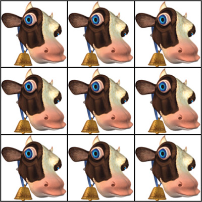
Note
The black border surrounding the tiled textures in Figure 5.8 is part of the actual texture and is not created as part of the wrapping process. This is included to help illustrate the integer boundaries where wrapping occurs.
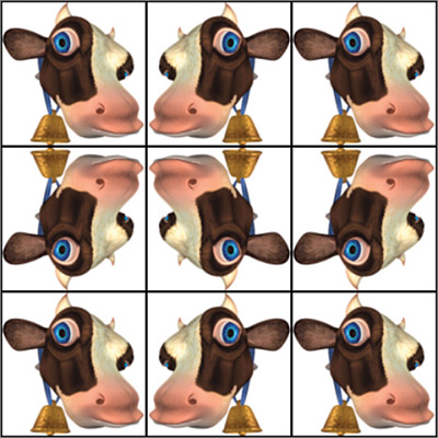
Mirror
Mirror address mode is similar to wrap mode, except that the texture is mirrored along integer boundaries instead of duplicated. Figure 5.9 shows the results of the same textured quad, but with mirror address mode enabled.
Clamp
In clamp address mode, the texture is not tiled. It is applied once, and all coordinates are clamped to the range [0, 1]. This has the effect of smearing the color of the texture’s edges, as in Figure 5.10.

Note
The mapped texture in Figure 5.10 is different than the texture in Figures 5.8 and 5.9. The black border has been removed and the image has been cropped so that the edge pixels vary in color. If the original texture had been used, the black border would be the color for every edge pixel and would be the “clamped” value.
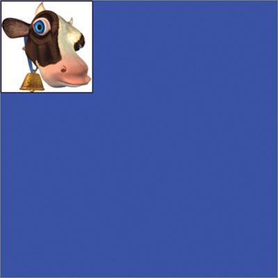
Border
As in clamp mode, border address mode applies the texture just once. But instead of smearing the edge pixels, a border color is used for all coordinates outside the range [0, 1]. Figure 5.11 shows the original, black-bordered cow texture, in border address mode with a blue border color.
Summary
In this chapter, you learned the details of texture mapping. You explored a complete texture mapping effect and uncovered additional HLSL syntax. You also learned about minification, magnification, mipmapping, and the filtering processes used to sample textures. Finally, you dove into the details of texture addressing modes and discovered how to produce various effects for geometry with texture coordinates that extend outside the range 0 to 1.
Texture mapping is fundamental to modern graphics, and future chapters build on this foundation.
Exercises
1. Modify the SamplerState object in TextureMapping.fx to experiment with various permutations of filter modes. Use point, linear, and anisotropic filtering, and observe the results as you zoom in and out with a textured surface.
2. Import a quad with UVs that range outside [0, 1], and experiment with the texture addressing modes in the SamplerState object of TextureMapping.fx. Specifically, use wrap, mirror, clamp, and border, and observe the results. The book’s companion website has an example quad (in .obj format, a 3D model format that NVIDIA FX Composer supports).