Appendix A
Historical Antecedents
In the beginning, there were data files… and from the need to manage the data stored in those files arose a variety of data management methods, most of which preceded the relational data model and, because of their shortcomings, paved the way for the acceptance of relational databases.
This appendix provides an overview of data management organizations used prior to the introduction of the relational data model. Although you do not need to read this appendix to understand the main body of this book, some of the case studies in Part III mention concepts discussed here. You will also find that NoSQL DBMSs (discussed in Chapter 28) share some characteristics with the older data models.
File Processing Systems
The first commercial computer—ENIAC—was designed to help process the 1960 census. Its designers thought that all computers could do was crunch numbers; the idea that computers could handle text data came later. Unfortunately, the tools available to handle data weren’t particularly sophisticated. In most cases, all the computing staff had available was some type of storage (at first tapes and later disks) and a high-level programming language compiler.
Early File Processing
Early file processing systems were made up of a set of data files—most commonly text files—and application programs that manipulated those files directly, without the intervention of a DBMS. The files were laid out in a very precise, fixed format. Each individual piece of data (a first name, a last name, street address, and so on) was known as a field. Those data described a single entity and were collected into a record. A data file was therefore made up of a collection of records.
Each field was allocated a specific number of bytes. The fixed field lengths meant that no delimiters were required between fields or at the end of records, although some data files did include them. A portion of such a data file might appear like Figure A.1.
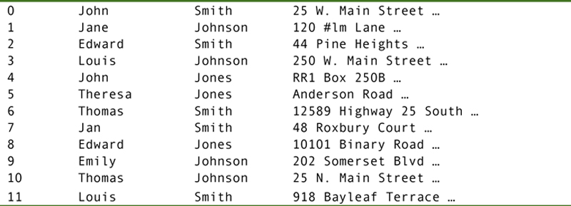
Figure A.1 A portion of a fixed field length data file.
The programs that stored and retrieved data in the data files located data by their byte position in the file. Assuming that the first record in a file was numbered 0, a program could locate the start of any field with the computation:

This type of file structure therefore was very easy to parse (in other words, separate into individual fields). It also simplified the process of writing the application programs that manipulated the files.
If the file was stored on tape, then access to the records was sequential. Such a system was well suited to batch processing if the records were in the order in which they needed to be accessed. If the records were stored on disk, then the software could perform direct access reads and writes. In either case, however, the program needed to know exactly where each piece of data was stored and was responsible for issuing the appropriate read and/or write commands.
Note: Some tape drives were able to read backwards to access data preceding the last written or read location. However, those that could not read backward needed to rewind completely and then perform a sequential scan beginning at the start of the tape to find data preceding the previous read/write location. Understandably, sequential access to data was unacceptably slow for interactive data processing.
These systems were subject to many problems, including all of those discussed in Chapter 3. In addition, programmers struggled with the following situations:
▪ Changing the layout of a data file (for example, changing the size of a field or record) required changing all of the programs that accessed that file, as well as rewriting the file to accommodate the new layout.
▪ Access was very fast when processing all records sequentially in the physical order of the file. However, searches for specific records based on some matching criteria also had to be performed sequentially, a very slow process. This held true even for files stored on disk.
The major advantage to a file processing system was that it was cheap. An organization that installed a computer typically had everything it needed: external storage and a compiler. In addition, a file processing system was relatively easy to create, in that it required little advance planning. However, the myriad problems resulting from unnecessary duplicated data, as well as the close coupling of programs and physical file layouts and the serious performance problems that arose when searching the file, soon drove data management personnel of the 1950s and 1960s to search for alternatives.
ISAM Files
Prior to the introduction of the database management system, programmers at IBM developed an enhanced file organization known as indexed sequential access method (ISAM), which supported quick sequential access for batch processing, but also provided indexes to fields in the file for fast access searches.
An ISAM file must be stored on disk. Initially, it is written to disk with excess space left in each cylinder occupied by the file. This allows records to be added in sequential key order. When a cylinder fills up, records are written to an overflow area and linked back to where they appear in the sequence in the file’s primary storage areas (see Figure A.2).
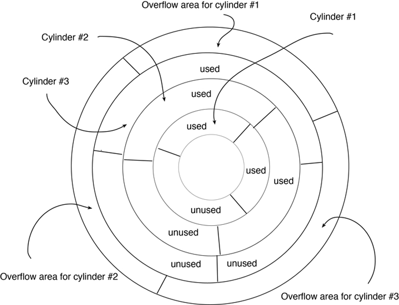
Figure A.2 ISAM file organization.
Note: Hard drives write files to a single track on a single surface in a disk drive. When the track is full, then the drive writes to the same track on another surface. The same tracks on all the surfaces in a stack of platters in a disk drive are known as a cylinder. By filling a cylinder before moving to another track on the same surface, the disk drive can avoid moving the access arm to which read/write heads are attached, thus saving time in the read or write process.
When the overflow area fills up, the file must be reblocked. During the reblocking process, the file size is increased and records are rewritten, once again leaving expansion space on each cylinder occupied by the file. No data processing can occur using the file while reblocking is in progress.
Depending on the implementation, indexes to ISAM files may be stored in the same file as the data or in separate files. When the data files are stored separately, the functions that manipulate the files treat the indexes and data as if they were one logical file.
Note: Although ISAM files have largely fallen into disuse, the DBMS Informix (now owned by IBM) continues to use its own version of ISAM—c-isam—for data storage.
Limitations of File Processing
File processing, regardless of whether it uses simple data files or ISAM files, is awkward at best. In addition to the problems mentioned earlier in this section, there are two more major drawbacks to file processing.
First, file processing cannot support ad hoc queries (queries that arise at the spur of the moment, cannot be predicted, and may never arise again). Because data files are created by the organization using them, there is no common layout to the files from one organization to another. There is therefore no reasonable way for a software developer to write a language that can query any data file; a language that could query file A probably wouldn’t work with file B because there is no similarity between the layout of the files. Therefore, access is limited to preplanned queries and reports that are provided by application programs.
So much of today’s data access requires ad hoc querying capabilities. Consider, for example, an ATM machine, perhaps the penultimate ad hoc query device. When you walk up to the machine, there is no way for the machine’s software to predict which account you will access. Nor is there any way to predict who will use a particular machine nor what that person will request from the machine. Therefore, the software must be able to access data at any time, from any location, from any account holder, and perform any requested action.
Second, when a file processing system is made up of many files, there is no simple way either to validate cross references between the files or to perform queries that require data from multiple files. This cross-referencing issue is a major data integrity concern. If you store customer data in file A and orders in file B, you want the customer data in file B (even if it’s only a customer number) to match the customer data in file B. Whenever data are duplicated, they must remain consistent. Unfortunately, when data are stored in multiple files, there is no easy way to perform this type of validation. The only way is to write a program that uses both files and explicitly verifies that the customer data in file B matches data in file A. Although this can certainly be done, file processing systems rarely perform this type of validation.
By the same token, queries or reports that require data to be extracted from multiple files are difficult to prepare. The application program that generates the output has to be created to read all necessary files, resulting in a program that is difficult to debug and maintain due to its complexity.
The solution is to look for some way to separate physical storage structures from logical data access. In other words, the program or user manipulating data shouldn’t need to be concerned about physical placement of data in files, but should be able to express data manipulation requests in terms of how data logically relate to one another. This separation of logical and physical data organization is the hallmark of a database system.
File Processing on the Desktop
One of the problems with data management software written for PCs has been that both developers and users often didn’t understand the exact meaning of the term database. As a result, the word was applied to any piece of software that managed data stored in a disk file, regardless of whether the software could handle logical data relationships.
The trend was started in the early 1980s by a product called pfs:File. The program was a simple file manager. You defined your fields and then used a default form for entering data. There was no way to represent multiple entities or data relationships. Nonetheless, the product was marketed as a database management system and the confusion in the marketplace began.
A number of products have fallen into this trap. One such product—FileMaker Pro—began as a file manager and has been upgraded to database status. The FileMaker company also introduced a product named Bento in 2008, which it advertised as a “personal database manager.” Bento was a rather nice piece of software, but it wasn’t a database management system; it was a file manager. After nearly 45 years, the confusion and the misuse of the term database persists.
You may often hear products such as those in the preceding paragraph described as “flat-file databases,” despite the term “database” being a misnomer. Nonetheless, desktop file managers can be useful tools for applications such as maintaining a mailing list, customer contact list, and so on.
The issue here is not to be a database snob, but to ensure that consumers actually understand what they are buying and the limitations that actually accompany a file manager. This means that you must pay special attention to the capabilities of a product when you are considering a purchase.
The Hierarchical Data Model
The first true database model to be developed was the hierarchical data model, which appeared as the basis of a commercial product in 1966. Like the two network data models that followed, it was a navigational data model, meaning that access paths were constrained by predeclared pointer structures in the schema.
Characteristics of the Hierarchical Data Model
A database that is designed to use the hierarchical data model is restricted to one-to-many relationships. In addition, no child entity may have more than one parent entity. The implications of this last restriction are significant.
As an example, consider the ER diagram in Figure A.3, which contains two hierarchies, or trees. The first relates departments to their employees and their projects. The second relates employees to projects. There is a one-to-many relationship between an employee and a department, but a many-to-many relationship between projects and employees. The relationship between department and project is one-to-may.
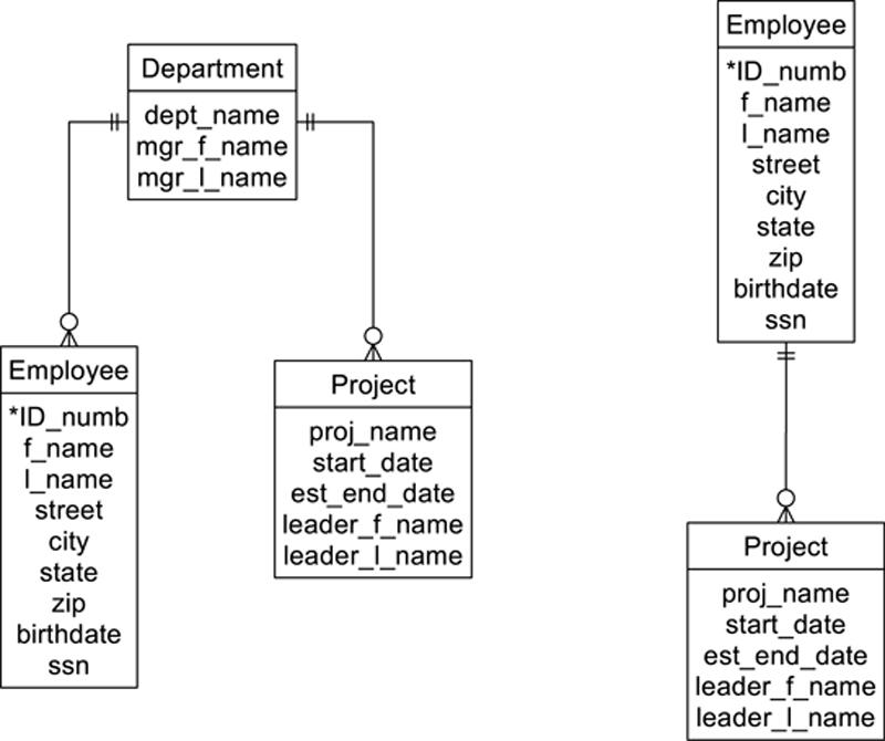
Figure A.3 Sample hierarchies.
Ideally, we would like to be able to use a composite entity to handle the many-to-many relationship. Unfortunately, the hierarchical data model does not permit the inclusion of composite entities. (There is no way to give a single entity two parent entities.) The only solution is to duplicate entity occurrences. This means that a project occurrence must be duplicated for every employee that works on the project. In addition, the project and employee entities are duplicated in the department hierarchy as well.
By their very nature, hierarchies include a great deal of duplicated data. This means that hierarchical databases are subject to the data consistency problems that arise from unnecessary duplicated data.
There is another major limitation to the hierarchical data model. Access is only through the entity at the top of the hierarchy, the root. From each root occurrence, the access path is top-down and left to right. This means that the path through the department hierarchy, for example, is through a department, to all its employees, and only then to the projects. For example, see Figure A.4, which contains two occurrences of the department/employee/project hierarchy. The arrows on the dashed lines represent the traversal order.
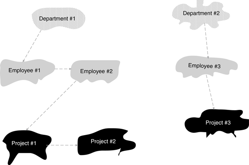
Figure A.4 Tree traversal order in two occurrences of a hierarchy.
The relationships between the entities in an occurrence of a hierarchy are maintained by pointers embedded in the data. As a result, traversing a hierarchy in its default order is very fast. However, if you need random access to data, then access can be extremely slow because you must traverse every entity occurrence in the hierarchy preceding a needed occurrence to reach the needed occurrence. Hierarchies are therefore well suited to batch processing in tree traversal order, but are not suitable for applications that require ad hoc querying.
The hierarchical model is a giant step forward from file processing systems, including those based on ISAM files. It allows the user to store and retrieve data based on logical data relationships. It therefore provides some independence between the logical and physical data storage, relieving application programmers to a large extent of the need to be aware of the physical file layouts.
IMS
The most successful hierarchical DBMS has been IMS, an IBM product. Designed to run on IBM mainframes, IMS has been handling high-volume transaction-oriented data processing since 1966. Today, IBM supports IMS legacy systems, but actively discourages new installations. In fact, many tools exist to help companies migrate from IMS to new products or to integrate IMS into more up-to-date software.
IMS does not adhere strictly to the theoretical hierarchal data mode. In particular, it does allow multiple parentage in some very restrictive situations. As an example, consider Figure A.5. There are actually two hierarchies in this diagram: the department to project hierarchy and the hierarchy consisting of just the employee.
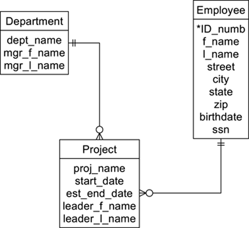
Figure A.5 Two IMS hierarchies with permitted multiple parentage.
Note: IMS refers to each hierarchy as a database and each entity as a segment.
The multiple parentage of the project entity is permitted because the second parent—the employee entity—is in another hierarchy and is at a higher level in the hierarchy. Despite the restrictions on multiple parentage, this easing of the rules goes a long way to removing unnecessary duplicated data.
IMS does not support a query language. All access is through application programs that are usually written in COBOL. Like a true hierarchical DBMS, it is therefore best suited to batch processing in tree traversal order. It has been heavily used in large businesses with heavy operational transaction processing loads, such as banks and insurance companies.
The Simple Network Data Model
At the same time IBM was developing IMS, other companies were working on DBMSs that were based on the simple network data model. The first DBMS based on this model appeared in 1967 (IDS from GE) and was welcomed because it directly addressed some of the limitations of the hierarchical data model. In terms of business usage, simple network databases had the widest deployment of any of the pre-relational data models.
Note: The network data models—both simple and complex—predate computer networks as we know them today. In the context of a data model, the term “network” refers to an interconnected mesh, such as a network of neurons in the brain or a television or radio network.
Characteristics of a Simple Network
A simple network database supports one-to-many relationship between entities. There is no restriction on multiple parentage, however. This means that the employees/departments/projects database we have been using as an example could be designed as in Figure A.6.
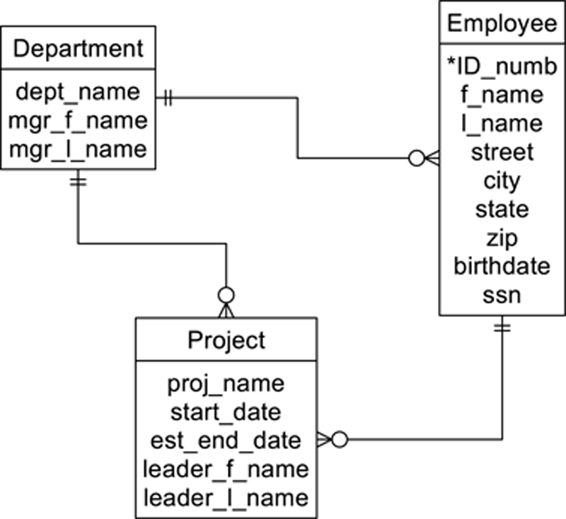
Figure A.6 A simple network data model.
In this example, the project acts as a composite entity between department and employee. In addition, there is a direct relationship between department and employee for faster access.
Given the restrictions of the hierarchical data model, the simple network was a logical evolutionary step. It removed the most egregious limitation of the hierarchical data model, that of no multiple parentage. It also further divorced the logical and physical storage, although as you will see shortly, simple network schemas still allowed logical database designers to specify some physical storage characteristics.
Simple network databases implement data relationships either by embedding pointers directly in the data or through the use of indexes. Regardless of which strategy is used, access to the data is restricted to the predefined links created by the pointers unless a fast access path has been defined separately for a particular type of entity. In this sense, a simple network is navigational, just like a hierarchical database.
There are two types of fast access paths available to the designer of a simple network. The first—hashing—affects the strategy used to place entity occurrences in a data file. When an entity occurrence is hashed into a data file, the DBMS uses a key (the value or one or more attributes) to compute a physical file locator (usually known as the database key). To retrieve the occurrence, the DBMS recomputes the hash value. Occurrences of related entities are then clustered around their parent entity in the data file. The purpose of this is twofold: It provides fast access to parent entities and puts child entities on the same disk page as their parents for faster retrieval. In the example we are using, a database designer might choose to hash department occurrences and cluster projects around their departments.
Note: A single entity occurrence can either be clustered or hashed; it can’t be both because the two alternatives determine physical placement in a data file.
The second type of fast access path is an index, which provides fast direct access to entity occurrences containing secondary keys.
If occurrences are not hashed and have no indexes, then the only way to retrieve them is by traversing down relationships with parent entity occurrences.
To enable traversals of the data relationships, a simple network DBMS must keep track of where it is in the database. For every program running against the database, the DBMS maintains a set of currency indicators, each of which is a system variable containing the database key of the last entity occurrence accessed of a specific type. For example, there are currency indicators for each type of entity, for the program as a whole, and so on. Application programs can then use the contents of the currency indicators to perform data accesses relative to the program’s previous location in the database.
Originally, simple network DBMSs did not support query languages. However, as the relational data model became more popular, many vendors added relational-style query languages to their products. If a simple network database is designed like a relational database, then it can be queried much like a relational database. However, the simple network is still underneath and the database is therefore still subject to the access limitations placed on a simple network.
Simple network databases are not easy to maintain. In particular, changes to the logical design of the database can be extremely disruptive. First, the database must be brought offline; no processing can proceed against it until the changes are complete. Once the database is down, then the following process occurs:
1. Back up all data or save the data in text files.
2. Delete the current schema and data files.
3. Compile the new database schema, which typically is contained in a text file, written in a data definition language (DDL).
4. Reallocate space for the data files.
5. Reload the data files.
In later simple network DBMSs, this process was largely automated by utility software, but considering that most simple network DBMSs were mainframe-based, they involved large amounts of data. Changes to the logical database could take significant amounts of time.
There are still simple network databases in use today as legacy systems. However, it would be highly unusual for an organization to decide to create a new database based on this data model.
CODASYL
In the mid-1960s, government and industry professionals organized into the Committee for Data Systems Languages (CODASYL). Their goal was to develop a business programming language, the eventual result of which was COBOL. As they were working, the committee realized that they had another output besides a programming language: the specifications for a simple network database. CODASYL spun off from the Database Task Group (DBTG), which in 1969 released its set of specifications.
The CODASYL specifications were submitted to the American National Standards Institute (ANSI). ANSI made a few modifications to the standard to further separate the logical design of the database from its physical storage layout. The result was two sets of very similar, but not identical, specifications.
Note: It is important to understand that CODASYL is a standard, rather than a product. Many products were developed to adhere to the CODASYL standards. In addition, there have been simple network DBMSs that employ the simple network data model but not the CODASYL standards.
A CODASYL DBMS views a simple network as a collection of two-level hierarchies known as sets. The database in Figure A.6 requires two sets: one for department → employee and department → project and the second for employee → project. The entity at the “one” end of the relationships is known as the owner of the set; entities at the “many” end of relationships are known as members of the set. There can be only one owner entity, but many member entities, of any set. The same entity can be an owner of one set and a member of another, allowing the database designer to build a network of many levels.
As mentioned in the previous section, access is either directly to an entity occurrence using a fast access path (hashing or an index) or in traversal order. In the case of a CODASYL database, the members of a set have an order that is specified by the database designer.
If an entity is not given a fast access path, then the only way to retrieve occurrences is through the owners of some set. In addition, there is no way to retrieve all occurrences of an entity unless all of those occurrences are members of the same set, with the same owner.
Each set provides a conceptual linked list, beginning with the owner occurrence, continuing through all member occurrences, and linking back to the owner. Like the occurrences of a hierarchy in a hierarchical database, the occurrences of a set are distinct and unrelated, as in Figure A.7.
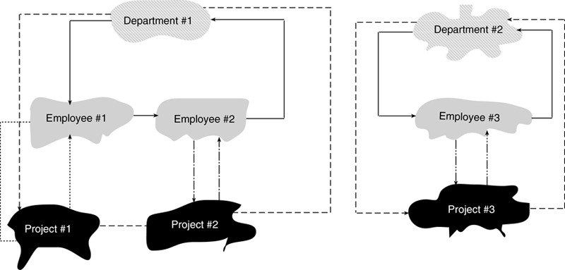
Figure A.7 Occurrences of CODASYL sets.
Note: Early CODASYL DBMSs actually implemented sets as linked lists. The result was complex pointer manipulation in the data files, especially for entities that were members of multiple sets. Later products represented sets using indexes, with database keys acting as pointers to the storage locations of owner and member records.
The independence of set occurrences presents a major problem for entities that aren’t a member of any set, such as the department occurrences in Figure A.7. To handle this limitation, CODASYL databases support a special type of set—often called a system set—that has only one owner occurrence, the database system itself. All occurrences of an entity that is a member of that set are connected to the single owner occurrence. Employees and projects would probably be included in a system set also to provide the ability to access all employees and all projects. The declaration of system sets is left up to the database designer.
Any DBMS that was written to adhere to either set of CODASYL standards is generally known as a CODASYL DBMS. This represents the largest population of simple network products that were marketed.
Arguably, the most successful CODASYL DBMS was IDMS, originally developed by Cullinet. IDMS was a mainframe product that was popular well into the 1980s. As relational DBMSs began to dominate the market, IDMS was given a relational-like query language and marketed as IDMS/R. Ultimately, Cullinet was sold to Computer Associates, which marketed and supported the product under the name CA-IDMS.
Note: Although virtually every PC DBMS in the market today claims to be relational, many are not. Some, such as FileMaker Pro, are actually simple networks. These are client/server products, robust enough for small business use. They allow multiple parentage with one-to-many relationships and represent those relationships with pre-established links between files. These are simple networks. This doesn’t mean that they aren’t good products, but simply that they don’t meet the minimum requirements for a relational DBMS.
The Complex Network Data Model
The complex network data model was developed at the same time as the simple network. It allows direct many-to-many relationships without requiring the introduction of a composite entity. The intent of the data model’s developers was to remove the restriction against many-to-many relationships imposed by the simple network data model. However, the removal of this restriction comes with a steep price.
There are at least two major problems associated with the inclusion of direct many-to-many relationships. Consider first the database segment in Figure A.8. Notice that there is no place to store data about the quantity of each item being ordered. The need to store relationship data is one reason why we replace many-to-many relationships with a composite entity and two one-to-many relationships.
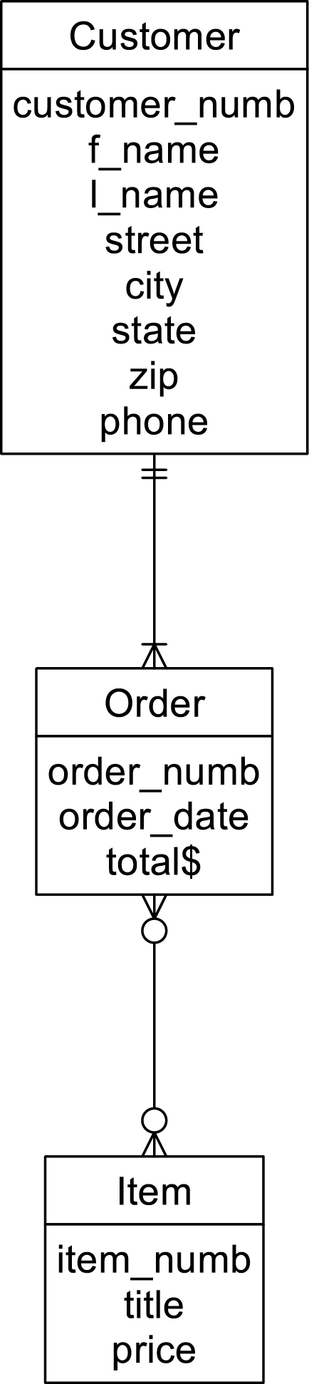
Figure A.8 A complex network lacking a place to store relationship data.
Nonetheless, if we examine an occurrence diagram for Figure A.8 (see Figure A.9), you can see that there is no ambiguity in the relationships. However, assume that we add another entity to the design, as in Figure A.10. In this case each item can appear on many shipments and each shipment can contain many items.
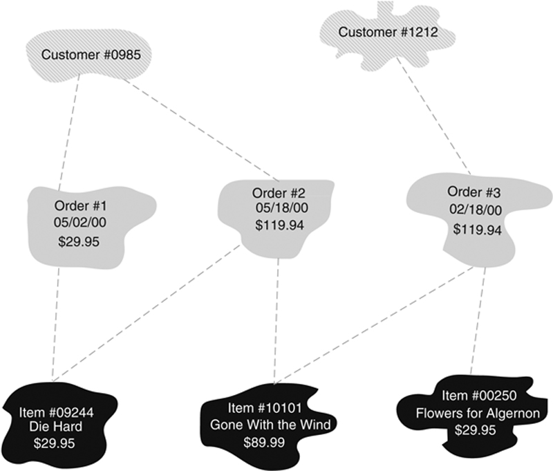
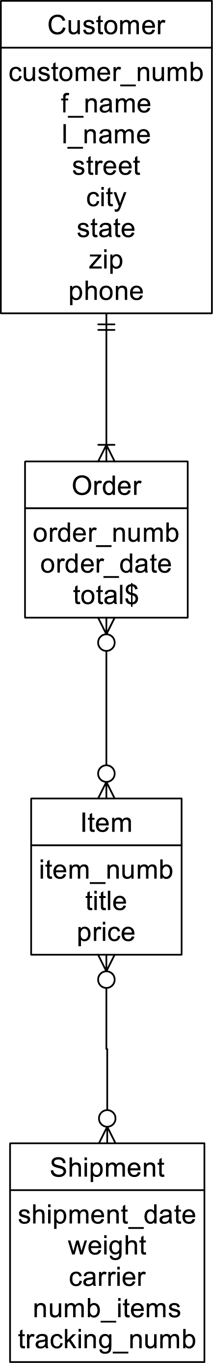
Figure A.10 A complex network with ambiguous logical relationships.
The problem with this design becomes clear when you look at the occurrences in Figure A.11. Notice, for example, that it is impossible to determine the order to which Shipment #1 and Shipment #2 belong. After you follow the relationships from the shipment occurrence to Item #1, there is no way to know which order is correct.
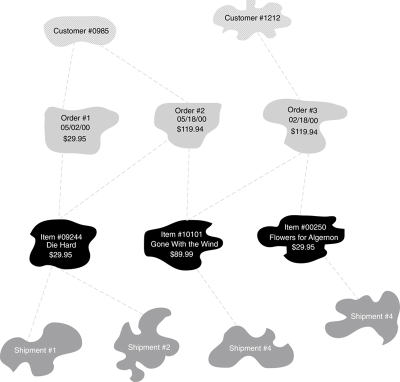
Figure A.11 Occurrences of the complex network in Figure A.10 containing ambiguous logical relationships.
There are two solutions to this problem. The first is to introduce an additional relationship to indicate which shipment comes from which order, as in Figure A.12. Although this is certainly a viable solution, the result is increased complexity for storing and retrieving data.
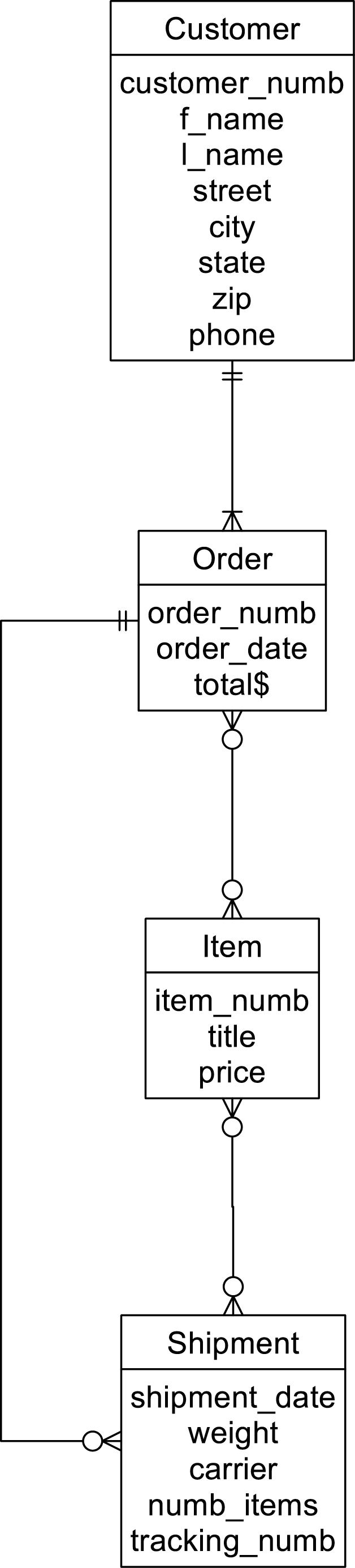
Figure A.12 Using an additional relationship to remove logical ambiguity in a complex network.
The other solution is to abandon the use of the complex network altogether and introduce composite entities to reduce all the many-to-many relationships to one-to-many relationships. The result, of course, is a simple network.
Note: A relational DBMS can represent all the relationships acceptable in a simple network—including composite entities—but does so in a non-navigational manner. Like a simple network, it can capture all of the meaning of a many-to-many relationship and still avoid data ambiguity.
Because of the complexity of maintaining many-to-many relationships and the possibility of logical ambiguity, there have been no widely successful commercial products based on the complex network data model. However, the data model remains in the literature, and provides some theoretical completeness to traditional data modeling.
..................Content has been hidden....................
You can't read the all page of ebook, please click here login for view all page.