
Chapter 3. Debugging AI Systems for Safety and Performance
Make sure that your AI models are validated and revalidated to ensure that they work as intended, and do not illegally discriminate.
— Using AI and Algorithms, United States Federal Trade Commission
For decades, error or accuracy on hold-out test data has been the standard by which machine learning (ML) models are judged. Unfortunately, as machine learning (ML) models are embedded into artificial intelligence (AI) systems that are deployed more broadly and for more sensitive applications, the standard approaches for ML model assessment have proven inadequate. For instance, test data area under the curve (AUC) tells us almost nothing about algorithmic discrimination, lack of transparency, privacy harms, or security vulnerabilities. Yet, these problems are often why AI systems fail once deployed. For acceptable in vivo performance, we simply must push beyond traditional in silica assessments designed primarily for research prototypes. Moreover, the best results for safety and performance occur when organizations are able to mix and match appropriate cultural competencies and process controls from Chapter 9 with AI technology that promotes trust. Chapter 15 presents sections on training, debugging, and deploying AI systems that delve into the numerous technical approaches for testing and improving safety, performance, and trust in AI.
Training
The discussion of training ML algorithms begins with reproducibility, because without that, it’s impossible to know if any one version of an AI system is really any better than another. Data and feature engineering will be addressed briefly and the training section closes by outlining key points for model specification.
Reproducibility
Without reproducibility, you’re building on sand. Reproducibility is fundamental to all scientific efforts, including AI. Without reproducible results, it’s very hard to know if day-to-day efforts are improving, or even changing, an AI system. Reproducibility helps ensure proper implementation and testing, and some customers may simply demand it. The techniques discussed below are some of the most common that data scientists and ML engineers use to establish a solid, reproducible foundation for their AI systems.
-
Benchmark Models: Benchmark models are important safety and performance tools for training, debugging, and deploying AI systems. They’ll be addressed several times in Chapter 15. In the context of model training and reproducibility, you should always build from a reproducible benchmark model. This allows a checkpoint for rollbacks if reproducbility is lost, but it also enables real progress. If yesterday’s benchmark is reproducible, and today’s gains above and beyond that benchmark are also reproducible, that’s real and measurable progress!
-
Hardware: As AI systems often leverage hardware acceleration via graphical processing units (GPUs) and other specialized system components, hardware is still of special interest for preserving reproducibility. If possible, try to keep hardware as similar as possible across development, testing, and deployment systems.
-
Environments: AI systems always operate in some computational environment, specified by the system hardware, system software, and your data and AI software stack. Changes in any of these can affect the reproducibility of ML outcomes. Thankfully, tools like Python virtual environments and Docker containers that preserve software environments have become commonplace in the practice of data science. Additional specialized environment management software from Domino Data Labs, gigantum, TensorFlow TFX, and Kubeflow can provide even more expansive control of computational environments.
-
Metadata: Data about data is essential for reproducibility. Track all artifacts associated with the model, e.g., datasets, preprocessing steps, model, data and model validation results, human sign offs, and deployment details. Not only does this allow rolling-back to a specific version of a dataset or model, but it also allows for detailed debugging and forensic investigations of AI incidents. For an open-source example of a nice tool for tracking metadata, checkout TensorFlow ML Metadata.
-
Random Seeds: Set by data scientists and engineers in specific code blocks, random seeds are the plow-horse of ML reproducibility. Unfortunately, they often come with language- or package-specific instructions. Seeds can take some time learn in different software, but when combined with careful testing, random seeds enable the building blocks of intricate and complex AI systems to retain reproducibility. This is a prerequisite for overall reproducibility.
-
Version Control: Minor code changes can lead to drastic changes in ML results. Changes to your own code plus it’s dependencies must be tracked in a professional version control tool for any hope of reproducibility. Git and GitHub are free and ubiquitous resources for software version control, but there are plenty of other options to explore. Crucially, data can also be version-controlled with tools like Pachyderm and DVC.
Though it may take some experimentation, some combination of these approaches and technologies should work to assure reproducibility in your AI system. Once this fundamental safety and performance control is in place, it’s time to consider other baseline factors like data quality and feature engineering.
Data Quality and Feature Engineering
Entire books have been written about data quality and feature engineering for ML and AI systems. This short subsection highlights some of the most critical aspects of this vast practice from a safety and performance perspective.
Starting with the basics, both the size and shape of a dataset are important safety and performance considerations. ML algorithms, that form the guts of today’s AI systems, are hungry for data. Both small data and wide, sparse data can lead to catastrophic performance failures in the real-world, because both give rise to scenarios in which system performance appears normal on test data, but is simply untethered to real-world phenomena. Small data can make it hard to detect underfitting, underspecification, overfitting, or other fundamental performance problems. Sparse data can lead to over-confident predictions for certain input values. If an ML algorithm did not see certain data ranges during training due to sparsity issues, most ML algorithms will issue a predictions in those ranges with no warning that the prediction is based on almost nothing.
A number of other data quality problems can cause safety worries, mostly due to misrepresentation of important information or propensity to cause overfitting or pipeline process issues. In Chapter 15, misrepresentation means data is distorted in a way that is consistent across training data partitions, but results in incorrect decisions once a model trained on the incorrect data is applied to new, live data. Overfitting refers to memorizing noise in training data and resulting optimistic error estimates, and pipeline issues are problems that arise from combining different stages of data preparation and modeling components into one prediction-generating executable. The short checklist below can be applied to most standard ML problems to help identify common data quality problems with safety and performance implications.
Misrepresentation
-
No duplicate data over-emphasizing unimportant information
-
No incorrect encoding or decoding of character or binary data
-
No incorrect use of time or date formats
-
Minimal one-hot encoding — reducing unnecessary sparsity
-
Minimal outliers — diminishing influence of outliers on model parameters or rules
-
Minimal use of simplistic imputation — preventing distortion of training distributions
-
Minimal correlation — increasing stability in model parameters or rules
-
Thorough normalization of character values — preventing mistreatment of modeled entities
Overfitting
-
No improper treatment of high cardinality categorical features
-
No naive target encoding
-
Minimal duplicate entities across training, validation, or test data partitions
-
Training data with time or date feature not split randomly for validation and testing
Pipeline Issues
-
All data cleaning and transformation steps applied during inference
-
Re-adjusting for over- or under-sampling during inference
Of course, many other problems can arise in data preparation and feature engineering, especially as the types of data that ML algorithms can accept for training becomes more varied. Applying the lens of misrepresentation, overfitting, or pipeline issues to think through how discrepancies in data or pipelines can lead to errors once the system is deployed is usually a helpful exercise for spotting pitfalls. Tools that detect and address such problems are also an important part of the the data science toolkit. For Python Pandas users, the pandas-profiling tool is a visual aide that helps to detect many basic data quality problems. R users also have options, as discussed by Mateusz Staniak and Przemysław Biecek in The Landscape of R Packages for Automated Exploratory Data Analysis.
Model Specification
Once your data preparation and feature engineering pipeline is hardened, it’s time to think about ML model specification. Considerations for real-world performance and safety are quite different from getting published or maximizing performance on ML contest leaderboards. While measurement of validation and test error remain important, bigger questions of accurately representing data and commonsense real-world phenomena have the highest priority. This subsection address model specification for safety and performance by highlighting the importance of benchmarks and alternative models, discussing the many hidden assumptions of ML models, and previewing the emergent disciplines of robust ML and ML safety and reliability.
Benchmarks and Alternatives
When starting a ML modeling task, it’s best to begin with a peer-reviewed training algorithm, and ideally to replicate any benchmarks associated with that algorithm. While academic algorithms rarely meet all the needs of complex business problems, starting from a well-known algorithm and benchmarks provides a baseline assurance that the training algorithm is implemented correctly. Once this sanity check is addressed, then think about tweaking a complex algorithm to address specific quirks of a given problem.
Along with comparison to benchmarks, evaluation of numerous alternative algorithmic approaches is another best practice that can improve safety and performance outcomes. The exercise of training many different algorithms and judiciously selecting the best of many options for final deployment typically results in higher-quality models because it increases the number of models evaluated and forces users to understand differences between them. Moreover, evaluation of alternative approaches is important in complying with a broad set of U.S. non-discrimination and negligence standards. In general, these standards require evidence that different technical options were evaluated and an appropriate trade-off between consumer protection and business need was made before deployment.
Hidden Assumptions
Like undetected misrepresentation problems in training data causing major problems once an AI system is deployed, ML algorithms that don’t align with fundamental structures in training data or in the real-world domain can cause serious incidents. Often times data scientists think they matched their models to the problem domain, but a wide array of hidden assumptions can still cause problems.
Selecting to use an ML algorithm for a modeling problem also comes with a lot of basic assumptions — essentially that high-degree interactions and nonlinearity in input features are important drivers of the predicted phenomenon. Conversely, choosing to use a linear model implicitly downplays interactions and nonlinearities. If those qualities are important for high-quality predictions, they’ll have to be specified explicitly for the linear model. In either case, it’s important to take stock of how main effects, correlations and local dependencies, interactions, nonlinearities, clusters, outliers, and hierarchies in training data, or in reality, will be handled by a modeling algorithm and to test those mechanisms. For optimal safety and performance once deployed, dependencies on time, geographical locations, or connections between entities must also be represented within ML models. Testing for independence of errors between rows in training data or plotting model residuals and looking for strong patterns are general and time-tested methods for ensuring such dependencies have been addressed. It is also possible to directly constrain ML algorithms to reflect reality. Monotonicity constraints ensure known monotonic relationships are reflected in ML models. Interaction constraints can prevent arbitrary or undesirable combinations of input features from affecting model predictions.
Another often unstated assumption that comes with many learning algorithms involves squared loss functions. Many ML algorithms use a squared loss function by default. This means your model thinks that your modeling target variable follows a normal distribution. Some modeling targets are normally distributed, but many are not. Matching your target distribution to your loss function is an important step in aligning your ML algorithm to the problem domain. Hyperparameters for ML algorithms are yet another place where hidden assumptions can cause safety and performance problems. Hyperparameters can be selected based on domain knowledge or via technical approaches like grid search and Bayesian optimization. The key is doing this process systematically and not assuming the large number of default settings in most ML algorithms will work for your data and your problem.
The Future of Safe and Robust Machine Learning
The new field of robust ML is churning out new algorithms with improved stability and security characteristics. Various researchers are creating new learning algorithms with guarantees for optimality, like optimal sparse decision trees. And researchers have put together excellent tutorial materials on ML safety and reliability. Today, these approaches require custom implementations and extra work, but hopefully soon these safety and performance advances will be more widely available.
Model Debugging
Once a model has been properly specified and trained, the next step in the technical safety and performance assurance process is testing and debugging. In years past, such assessments focused on accuracy and error rates in holdout data. As ML models are incorporated in public-facing AI systems, and the number of publicly reported AI incidents is increasing dramatically, it’s clear that more rigorous validation is required. The new field of model debugging is rising to meet this need. Model debugging treats ML models more like code and less like abstract mathematics. It applies a number of different testing methods to find software flaws, logical errors, inaccuracies, and security vulnerabilities in ML models and AI system pipelines. Of course, these bugs must also be fixed when they are found. This section of Chapter 15 explores model debugging in some detail, starting with basic and traditional approaches, moving onto specialized testing techniques, delineating the common bugs we’re trying to find, and closing with a discussion of bug remediation methods.
Software Testing
Basic software testing becomes much more important when we stop thinking of pretty figures and impressive tables of results as the end goal of an ML model training task. When AI systems are deployed, they need to work correctly under various circumstances. Almost more than anything else related to AI and ML systems, making software work is an exact science. Best practices for software testing are well-known and can even be made automatic in many cases. At a minimum, mission-critical AI systems should undergo:
-
Unit testing: All functions, method, subroutines or other code blocks should have tests associated with them to ensure they behave as expected, accurately, and are reproducible. This ensures the building blocks of an AI system are solid.
-
Integration testing: All APIs and interfaces between modules, tiers, or other subsystems should be tested to ensure proper communication. API mismatches after backend code changes are a classic failure mode for AI systems. Use integration testing to catch this and other integration fails.
-
Functional Testing: Functional testing should be applied to AI system user interfaces and endpoints to ensure that they behave as expected once deployed.
-
Chaos Testing: Testing under chaotic and adversarial conditions can lead to better outcomes when your AI systems faces complex and surprising in vivo scenarios.
Two additional ML-specific tests should be added into the mix to increase quality further:
-
Random Attack: Random attacks expose AI systems or ML models to vast amounts of random data to catch both software and math problems. The real world is a chaotic place. Your AI system will encounter data for which it’s not prepared. Random attacks can decrease those occurrences and any associated glitches or incidents.
-
Benchmarking: Use benchmarks to track system improvements over time. AI systems can be incredibly complex. How can you know if the 3 lines of code an engineer changes today made a difference in the performance of the system as a whole? If system performance is reproducible, and benchmarked before and after changes, it’s much easier to answer such questions.
ML is software. So, all the testing that’s done on traditional enterprise software assets should be done on important AI systems as well. If you don’t know where to start with modeling debugging, start with random attack. You may very well be shocked at the math or software bugs random data can expose in your systems. When you add benchmarks to your organization’s continuous integration/continuous development (CI/CD) pipelines, that’s the another big step toward assuring the safety and performance of AI systems.
Traditional Model Assessment
Once you feel confident that the code in your AI systems is functioning as expected, it’s easier to concentrate on testing the math of your ML algorithms. Looking at standard performance metrics is important. But it’s not the end of the validation and debugging process — it’s the beginning. While exact values and decimal points matter, from a safety and performance standpoint, they matter much less than they do on the leaderboard of an ML contest. When considering in-domain performance, it’s less about exact numeric values of assessment statistics, and more about mapping in silica performance to in vivo performance.
If possible, try to select assessment statistics that have a logical interpretation and practical or statistical thresholds. For instance, root mean squared error (RMSE) can be calculated for many types of prediction problems, and crucially, it can be interpreted in units of the target variable. Area under the curve (AUC), for classification tasks, is bounded between 0.5 at the low end and 1.0 at the high end. Such assessment measures allow for commonsense interpretation of ML model performance and for comparison to widely accepted thresholds for determining quality. It’s also important to analyze performance metrics across important segments in your data and across training, validation, and testing data partitions. When comparing performance across segments within training data, it’s important that all those segments exhibit roughly equivalent and high quality performance. Amazing performance on one large customer segment, and poor performance on everyone else, will look fine in average assessment statistic values like RMSE. But, it won’t look fine if it leads to public brand damage due to many unhappy customers. Varying performance across segments can also be a sign of underspecification, a serious ML bug that will be addressed in more detail later in Chapter 15. Performance across training, validation and test datasets are usually analyzed for under and overfitting. Like underspecification, these are serious bugs that will receive more detailed treatment below.
Another practical consideration related to traditional model assessment is selecting a probability cutoff threshold. Most ML models for classification generate numeric probabilities, not discrete decisions. Selecting the numeric probability cutoff to associate with actual decisions can be done in various ways. While it’s always tempting to maximize some sophisticated assessment measure, it’s also a good idea to consider real-world impact. Let’s consider a classic lending example. Say a probability of default model threshold is originally set at 0.15, meaning that everyone who scores less than a 0.15 probability of default is approved for a loan, and those that score at the threshold or over are denied. Think through questions like:
-
What is the expected monetary return for this threshold?
-
What is the risk?
-
How many people will get the loan at this threshold?
-
How many women? How many minority group members?
Outside of the probability cutoff thresholds, it’s always a good idea to estimate in-domain performance, because that’s what we really care about. Assessment measures are nice, but what matters is making money versus losing money, or even saving lives versus taking lives. You can take a first crack at understanding real-world value by assigning monetary, or other, values to each cell of a confusion matrix for classification problems or to each residual unit for regression problems. Do a back-of-the-napkin calculation. Does it look like your model will make money or lose money? Once you get the gist of this kind of valuation, you can even incorporate value levels for different model outcomes directly into ML loss functions, and optimize towards the best-suited model for real-world deployment.
Error and accuracy metrics will always be important for ML. But once ML algorithms are used in deployed AI systems, numeric values and comparisons matter less than they do for publishing papers and playing Kaggle. So, keep using traditional assessment measures, but try to map them to in-domain safety and performance.
Residual Analysis for Machine Learning
Residual analysis is another type of traditional model assessment that can be highly effective for ML models and AI systems. At it’s most basic level, residual analysis means learning from mistakes. That’s an important thing to do in life, as well as in organizational AI systems. Moreover, residual analysis is a tried and true model diagnostic technique. This subsection will use an example and three generally applicable residual analysis techniques to apply this established discipline to ML.
Example Setup
Since residual analysis is a fairly technical topic, we’ll use an example problem and some related figures for clarity’s sake. The figures below are based on the well-known Taiwanese credit card dataset from the University of California Irvine (UCI) ML repository. In this dataset, the object is to predict if someone will pay, DEFAULT_NEXT_MONTH = 0, or default, DEFAULT_NEXT_MONTH = 1, on their next credit card payment. Features about payments are used to generate probabilities of default, or p_DEFAULT_NEXT_MONTH. The example ML model is trained on payment features including PAY_0 — PAY_6, or a customer’s most recent through six months prior repayment statuses (higher values are late payments), PAY_AMT1 — PAY_AMT6, or a customer’s most recent through six months prior payment amounts, and BILL_AMT1 — BILL_AMT6, or a customer’s most recent through six months prior bill amounts. All monetary values are reported in Taiwanese Dollars (NT$).
Some of the figures also contain the features LIMIT_BAL and r_DEFAULT_NEXT_MONTH. LIMIT_BAL is a customer’s credit limit. r_DEFAULT_NEXT_MONTH is a logloss residual value, or a numeric measure of how far off the prediction, p_DEFAULT_NEXT_MONTH, is from the known correct answer, DEFAULT_NEXT_MONTH. You may also see demographic features in the dataset, like SEX, that are used for bias testing. For the most part, Chapter 15 treats the example credit lending problem as a general predictive modeling exercise, and does not consider applicable regulations.
Analysis and Visualizations of Residuals
Plotting residuals and examining them for tell-tale patterns of different kinds of problems is a long-running model diagnostic technique. And it can be applied to ML algorithms to great benefit with a bit of creativity and elbow grease. Simply plotting residuals for an entire dataset can be helpful, especially to spot outlying rows causing very large numeric errors or to analyze overall trends in errors. However, breaking residual values and plots down by feature and level, as illustrated in Figure 1, is likely to be more informative. In the top row of Figure 1, favorable values for PAY_0, -2,-1,0 representing paying on time or not using credit, are associated with large residuals for customers who default. In the bottom rows the exact opposite, but still obvious, behavior is displayed. Customer’s with unfavorable values for PAY_0 cause large residuals when they suddenly pay on time. What’s the lesson here? Figure 1 shows that the ML model in question would make the same mistakes a human, or a simple business rule, would make. Now that we know about these simplistic decision processes, which happen to arise from thousands of machine-learned rules, the model can be improved, or just replaced with a more transparent and secure business rule: IF PAY_0 < 2 THEN APPROVE, ELSE DENY.

Figure 3-1. Residuals show that a model makes the same obvious mistakes a human might. Customers with good payment track records who default suddenly cause large residuals, as do customers with poor payment track records who suddenly start paying on time. Adapted from Responsible Machine Learning with Python.
Do you have a lot features or features with many categorical levels? You’re not off the hook! Start with the most important features and their most common levels. Residual analysis is considered standard practice for important linear regression models. ML models are arguably higher-risk and more failure prone, so they need even more residual analysis and model debugging.
Modeling Residuals
Modeling residuals with interpretable models is another great way to learn more about the mistakes your AI system could make. Figure 2 displays a decision tree model of the example ML model’s residuals for DEFAULT_NEXT_MONTH = 1, or customer’s who default. While it reflects what was discovered in Figure 1, it does so in a very direct way that exposes the logic of the failures. In fact, it’s even possible to build programmatic rules about when the model is likely to fail the worst. The worst residuals occur when: PAY_0 < 0.5 AND PAY_AMT2 >= 2802.5 AND PAY_4 < 1 AND LIMIT_BAL >= 256602.0 Or more plainly, this model fails when a customer exhibits excellent payment behavior, but then suddenly defaults.
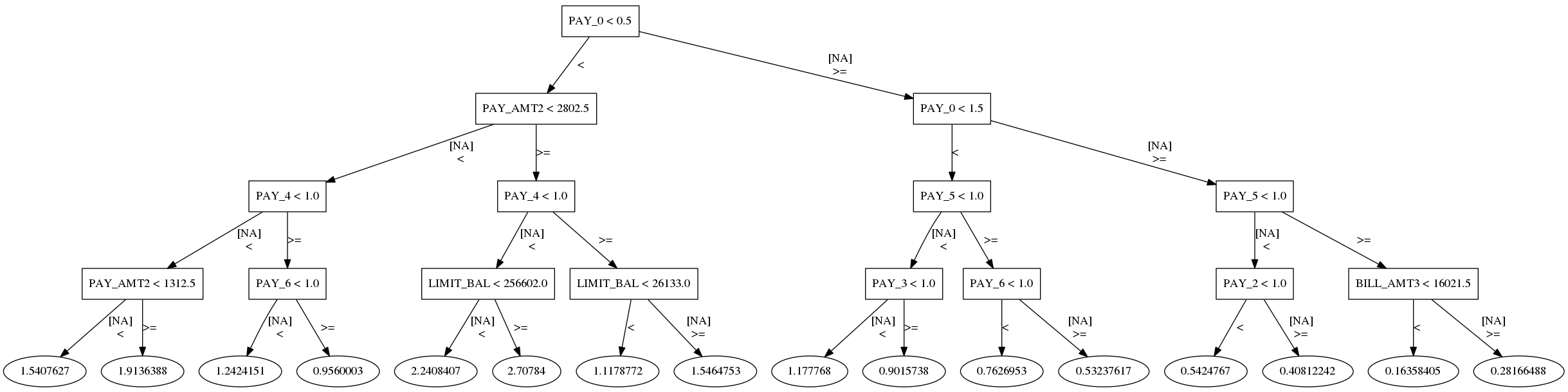
Figure 3-2. An interpretable decision tree model of the example ML model’s residuals displays patterns that can be used to spot failure modes and design mitigation approaches. Adapted from Responsible Machine Learning with Python.
In general this technique helps uncover failure modes. Once failure modes are known, they can be mitigated to increase performance and safety. For the example, if the patterns in Figure 4 can be isolated from patterns that result in non-default, this can lead to precise remediation strategies in the form of model assertions. Model assertions, also known as business rules, are a mitigation technique that can be applied directly to ML model predictions to address such discovered failure modes. Model assertions will be discussed in greater detail below, but don’t be shy about applying other common sense actions to increase safety and performance.
Local Contribution to Residuals
Plotting and modeling residuals are older techniques that are well-known to skilled practitioners. A more recent breakthrough has made it possible to calculate accurate Shapley value contributions to model errors! This means for any feature or row of any dataset, we can now know which features are driving model predictions, and which features are driving model errors. What this advance really means for ML is yet to be determined, but the possibilities are certainly intriguing. One obvious application for this new Shapley value technique is to compare feature importance for predictions to feature importance for residuals, as illustrated in Figure 3.
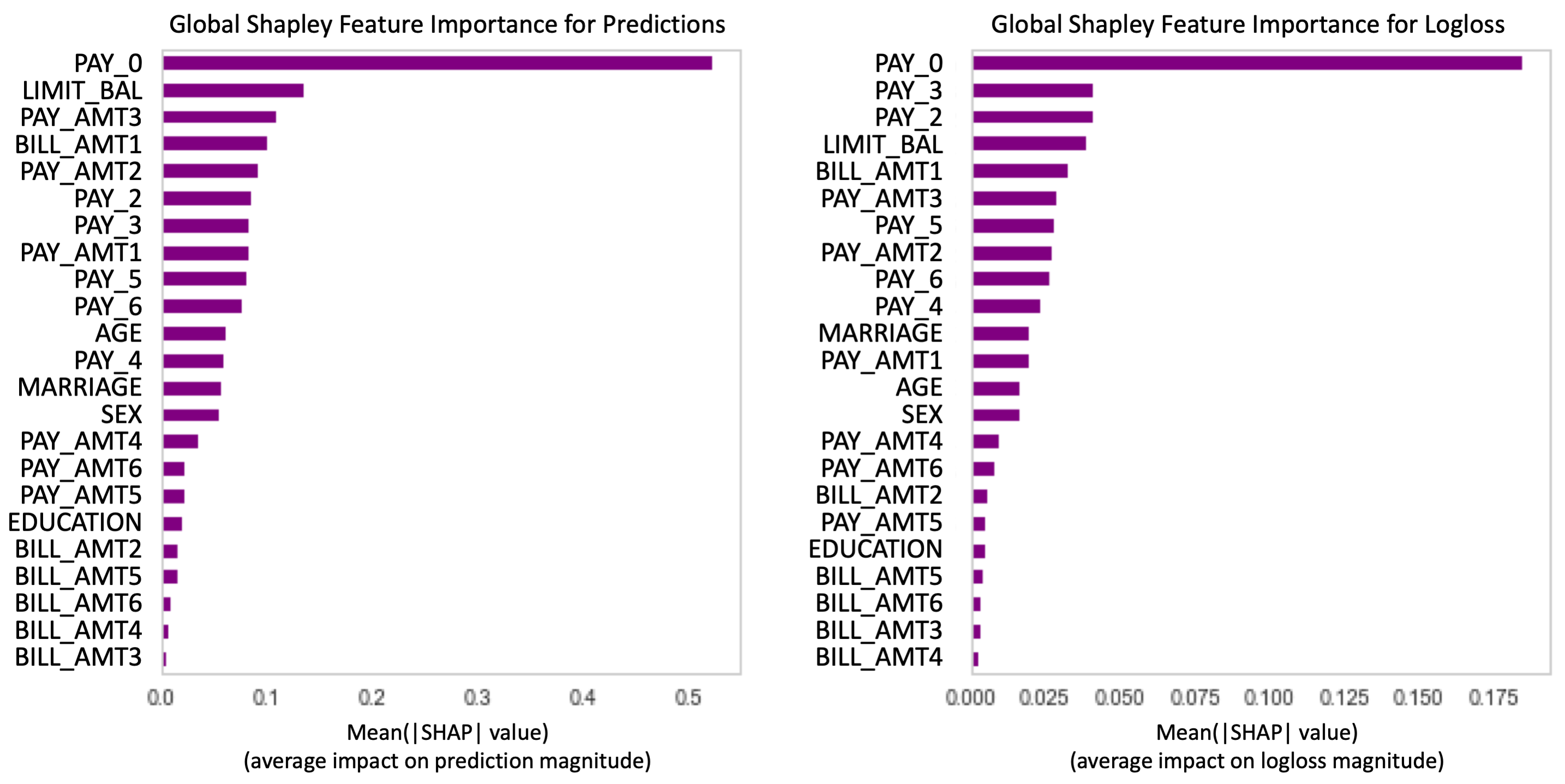
Figure 3-3. It is now possible to calculate Shapley value contributions to model errors! This means we can know which features are driving predictions, which features are driving errors, and consider mitigation approaches for non-robust features that contribute more to errors than to predictions. Adapted from Responsible Machine Learning with Python.
Figure 3 shows accurate Shapley value feature importance on the left, and accurate Shapley values contributions to residuals on the right, both aggregated over an entire dataset. This reveals that non-robust features like PAY_2 and PAY_3 are actually more important to model residuals than model predictions! Meaning these features should be examined carefully, have strong regularization or noise injection applied to them, or even be dropped from the analysis.
This ends our brief tour of residual analysis for ML. Of course there are other ways to study the errors of ML models. If you prefer another way, then go for it! The important thing is do some kind of residual analysis for all high-stakes AI systems. Along with sensitivity analysis, to be discussed in the next subsection, residual analysis is a major component of the toolkit for ML model debugging.
Sensitivity Analysis
Unlike linear models, it’s very hard to understand how ML models extrapolate or perform on new data, without testing them explicitly. That’s the simple and powerful idea behind sensitivity analysis. Find or simulate data for interesting scenarios, then see how your model performs on that data. You really won’t know how your AI system will perform in these scenarios unless you do basic sensitivity analysis. Of course, there are structured and more efficient variants of sensitivity analysis, such as in the interpret library from Microsoft Research. Another great option for sensitivity analysis, and a good place to start with more advanced model debugging techniques is random attacks, discussed in the Software Testing subsection. Many other approaches, like stress-testing, visualization, and adversarial example searches also provide standardized ways to conduct sensitivity analysis.
-
Stress-Testing: Stress-testing involves simulating data that represents realistic adverse scenarios, like recessions or pandemics, and making sure your ML models and any downstream business processes will hold up to the stress of the adverse situation.
-
Visualizations: Visualizations like plots of accumulated local affect (ALE), individual conditional local effect (ICE), and partial dependence curves are a well-known and highly structured way to observe the performance of ML algorithms across various real or simulated values of input features.
-
Adversarial Example Searches: Adversarial examples are rows of data that evoke surprising responses from ML models. Deep learning approaches can be used to generate adversarial examples for unstructured data, and ICE and genetic algorithms can be used to generate adversarial examples for structured data. Adversarial examples, and searching for them, are a great way to find local areas in your ML response functions or decision boundaries that can cause incidents once deployed.
Figure 4 shows the results of combining visualizations and adversarial example searches in model debugging. The response surfaces in Figure 4 were formed by randomly perturbing a certain interesting row of data many thousands of times and plotting the associated predictions. How was this interesting row of data selected for the basis of an adversarial example search? ICE. The surfaces are based on an ICE curve that showed a particularly drastic swing for different values of input variables.
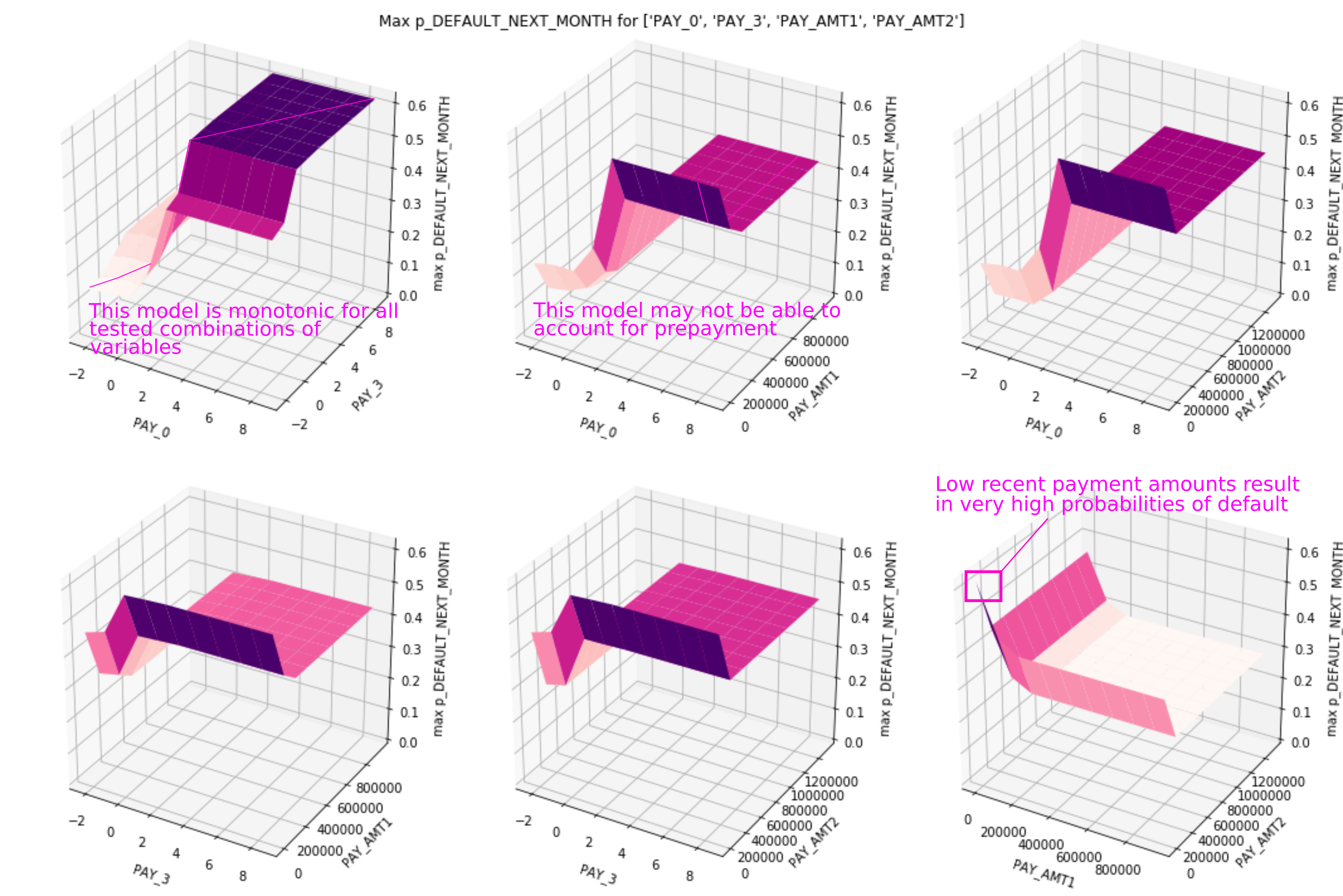
Figure 3-4. Adversarial example search shows several interesting positive and negative results.
Getting back to the example data and ML model discussed in previous sections, Figure 4 shows the results of six adversarial example searches, seeded by an ICE curve, and presents some positive and negative findings. On the positive side, each response surface shows monotonicity. These simulations confirm that monotonic constraints, supplied at training time and based on domain knowledge, held up during training. On the negative side, a potential logical flaw and a vulnerability to adversarial attack were also discovered. According to one of the response surfaces, the example model will issue high probability of default predictions once customers become two months late on their most recent payment (PAY_0). This harsh treatment is applied even in the circumstance where a customer repays (PAY_AMT1) over their credit limit. This potential logical flaw could prevent pre-payment or over-penalize good customers who failed pay their bill while on vacation. Another surface also shows a surprisingly steep spike in predictions for low first (PAY_AMT1) and second payment (PAY_AMT2) values. This could present an avenue for adversarial examples to evoke surprisingly high probability of default predictions once the system is deployed.
Each of the discussed sensitivity analysis approaches and the example adversarial search technique can provide insight into how your AI system might perform when it encounters certain kinds of data in the real world. A theme of Chapter 15 is anticipating how an AI system will perform in the real-world and making sure it’s performance in the lab is relevant to it’s in vivo performance, so that appropriate controls can be applied before deployment. Sensitivity analysis is one of most direct tools for simulating real-world performance and making sure your AI system is ready for what it may face once deployed.
Benchmark Models
Benchmark models have been discussed at numerous points within 15. They are a very important safety and performance tool, with uses throughout the AI lifecycle. This subsection will discuss benchmark models in the context of model debugging and also summarize other critical uses.
The first way to use a benchmark model for debugging is to compare performance between a benchmark and the AI system in question. If the AI system does not outperform a simple benchmark, and many may not, it’s back to the drawing board! Assuming a system passes this initial baseline test, benchmark models are a comparison tool used to interrogate mechanisms and find bugs within an AI system. For instance, data scientists can ask the question: “which predictions does my benchmark get right and my AI system get wrong?” Given that the benchmark should be well understood, it should be clear why it is correct, and this understanding should also provide some clues as to what the AI system is getting wrong. Benchmarks can also be used for reproducibility and model monitoring purposes as follows:
Reproducibility Benchmarks: Before making changes to a complex AI system it is imperative to have a reproducible benchmark from which to measure performance gains, or losses. A reproducible benchmark model is an ideal tool for such measurement tasks. If this model can be built into CI/CD processes that enable automated testing for reproducibility and comparison of new system changes to established benchmarks, even better!
Debugging Benchmarks: As discussed above, comparing complex ML model mechanisms and predictions to a trusted, well-understood benchmark model’s mechanisms and predictions is an effective way to spot ML bugs.
Monitoring Benchmarks: Comparing real-time predictions between a trusted benchmark model and a complex AI system is a way to catch serious ML bugs in real-time. If a trusted benchmark model and a complex AI system give noticeably different predictions for the same instance of new data, this can be a sign of an ML hack, data drift, or even algorthmic discrimination. In such cases, benchmark predictions can be issued in place of AI system predictions, or predictions can be withheld until human analysts determine if the AI system prediction is valid.
If you set benchmarks up efficiently, it may even be possible to use the same model for all three tasks. A benchmark can be run before starting work to establish a baseline from which to improve performance, and that same model can be used in comparisons for debugging and model monitoring. When a new version of the system outperforms an older version in a reproducible manner, the ML model at the core of the system can become the new benchmark. If your organization can establish this kind of workflow, you’ll be benchmarking and iterating your way to increased AI safety and performance.
Machine Learning Bugs
Now that we know how to find ML bugs with software QA, traditional model assessment, residual analysis, sensitivity analysis and benchmark models, what exactly are we looking for? As discussed elsewhere in 15, there’s a lot that can go wrong, and thinking about an AI system’s operating environment is key to understanding failure modes. But when it comes to the math of ML, there are a few emergent gotchas and many well-known pratfalls. This subsection will discuss some usual suspects and some dark horse bugs including distributional shifts, instability, looped inputs, overfitting, underfitting, and underspecification.
Distributional Shifts
Shifts in the underlying data between different training data partitions and after model deployment are common failure modes for AI systems. Whether it’s a new competitor entering a market or a devastating world-wide pandemic, the world is a dynamic place. Unfortunately most of today’s AI systems learn patterns from static snapshots of training data and try to apply those patterns in new data. Sometimes that data is holdout validation or testing partitions. Sometimes it’s live data in a production scoring queue. Regardless, drifting distributions of input features is a serious bug that must be caught and squashed. (Before you jump to the conclusion that adaptive, on-line, or reinforcement learning AI systems will solve the problem of distributional drift, I’d like to point out that such systems currently implicate untenable risks for in vivo instability and insecurity.) When training ML models, watch out for distributional shifts between training, cross-validation, validation, or test sets using KS-, t-, or other appropriate statistical tests. If a feature has a different distribution from training partition to another, drop it or regularize it heavily. Another smart test for distributional shifts to conduct during debugging is to simulate distributional shifts for potential deployment conditions. Worried about how your model will perform during a recession? Simulated distributional shifts to simulate more late payments, lower cash flow, and higher credit balances and see how your model performs. It’s also crucial to record information about distributions in training data so that drift after deployment can be detected easily.
Instability
ML models can exhibit instability in the training process or when making predictions on live data. Instability in training is often related to small training data, sparse regions of training data, highly correlated features within training data, or high-variance model forms, such as deep single decision trees. Cross-validation is a typical tool for detecting instability during training. If a model displays noticeably different error or accuracy properties across cross-validation folds then you have an instability problem. Training instability can often be remediated with better data and lower-variance model forms such as decision tree ensembles. Plots of ALE or ICE also tend to reveal prediction instability in sparse regions of training data, and instability in predictions can be analyzed using sensitivity analysis: simulations, stress-testing, and adversarial example searches. If probing your response surface or decision boundary with these techniques uncovers wild swings in predictions, or your ALE or ICE curves are bouncing around, especially in high or low ranges of feature values, you also have an instability problem. This type of instability can often be fixed with constraints and regularization.
Looped Inputs
As AI systems are incorporated into broader digitalization efforts, or implemented as part of larger decision support efforts, multiple data-driven systems often interact. In these cases, error propagation and feedback loop bugs can occur. Error propagation occurs when small errors in one system cause or amplify errors in another system. Feedback loops are a way an AI system can fail by being right. Feedback loops occur when an AI system affects its environment and then those effects are re-incorporated into system training data. Examples of feedback loops include when predictive policing leads to over-policing of certain neighborhoods or when employment algorithms intensify diversity problems in hiring by continually recommending correct, but non-diverse, candidates. Dependencies between systems must be documented and deployed models must be monitored so that debugging efforts can detect error propagation or feedback loop bugs.
Leakage
Information leakage between training, validation, and test data partitions happens when information from validation and testing partitions leaks into a training partition, resulting in overly optimistic error and accuracy measurements. Leakage can happen for a variety of reasons, including:
-
Feature Engineering: If used incorrectly, certain feature engineering techniques such as imputation or principal components analysis (PCA) may contaminate training data with information from validation and test data. To avoid this kind of leakage, perform feature engineering uniformly, but separately, across training data partitions. Or ensure that information, like means and modes used for imputation, are calculated in training data and applied to validation and testing data, and not vice-versa.
-
Mistreatment of Temporal Data: Don’t use the future to predict the past. Most data has some association with time, whether explicit as in time-series data, or some other implicit relationship. Mistreating or breaking this relationship with random sampling is a common cause of leakage. If you’re dealing with data where time plays a role, time needs to be used in constructing model validation schemes. The most basic rule is that the earliest data should be in training partitions while later data should be divided into validation and test partitions, also according to time.
-
Multiple Identical Entities: Sometimes the same person, financial or computing transaction, or other modeled entity will be in multiple training data partitions. When this occurs, care should be taken to ensure that ML models do not memorize characteristics of these individuals then apply those individual-specific patterns to different entities in new data.
Keeping an untouched, time-aware holdout set for an honest estimate of real-world performance can help with many of these different leakage bugs. If error or accuracy on such a holdout set looks a lot less rosy than on partitions used in model development, you might have a leakage problem. More complex modeling schemes involving stacking, gates, or bandits can make leakage much harder to prevent and detect. However, a basic rule of thumb still applies: do not use data involved in learning or model selection to make realistic performance assessments. Using stacking, gates, or bandits means you need more holdout data for the different stages of these complex models to make an accurate guess at in vivo quality. More general controls such as careful documentation of data validation schemes and model monitoring in deployment are also necessary for any AI system.
Overfitting
Overfitting happens when a complex ML algorithm memorizes too much specific information from training data, but does not learn enough generalizable concepts to be useful once deployed. Overfitting is often caused by high-variance models, or models that are too complex for the data at hand. Overfitting usually manifests in much better performance on training data than on validation, cross-validation, and test data partitions. Since overfitting is a ubiquitous problem, there are many possible solutions, but most involve decreasing the variance in your chosen model. Examples of these solutions include:
-
Ensemble Models: Ensemble techniques, particularly bootstrap aggregation (i.e., bagging) and gradient boosting are known to reduce error from single high-variance models. So, try one of these ensembling approaches if you encounter overfitting. Just keep in mind that when switching from one model to many, you can decrease overfitting and instability but you’ll also likely loose interpretability.
-
Reducing Architectural Complexity: Neural networks can have too many hidden layers or hidden units. Ensemble models can have to many base learners. Trees can be too deep. If you think you’re observing overfitting, make your model architecture less complex.
-
Regularization: Regularization refers to many sophisticated mathematical approaches for reducing the strength, complexity, or number of learned rules or parameters in an ML model. In fact, many types of ML models now incorporate multiple options for regularization, so make sure you employ these options to decrease the likelihood of overfitting.
-
Simpler Hypothesis Model Families: Some ML models will be more complex than others out-of-the-box. If your neural network or gradient boosting machine (GBM) look to be overfit, you can try a less complex decision tree or linear model.
Overfitting is traditionally seen as the Achilles’ heal of ML. While it is one the most likely bugs to encounter, it’s also just one of many possible technical risks to consider from a safety and performance perspective. As with leakage, as ML systems become more complex, overfitting becomes harder to detect. Always keep an untouched holdout set with which to estimate real-world performance before deployment. More general controls like documentation of validation schemes, model monitoring, and A/B testing of models on live data also need to be applied to prevent overfitting.
Shortcut Learning
Shortcut learning occurs when a complex AI system is thought to be learning and making decisions about one subject, say anomalies in lung scans or job interview performance, but it’s actually learned about some simpler related concept, such as machine identification numbers or Zoom video call backgrounds. Use interpretable models and explainable AI (XAI) techniques to understand what learned mechanisms are driving model decisions, and make sure you understand how your AI system makes decisions.
Underfitting
If someone tells you a statistic about a set of data, you might wonder how much data that statistic is based on, and whether that data was of high enough quality to be trustworthy. What if someone told you they had millions, billions, or even trillions of statistics for you, they would need lots of data to make a case that all these statistics were meaningful. Just like averages and other statistics, each parameter or rule within an ML model is learned from data. Big ML models need lots of data to learn enough to make their millions, billions, or trillions of learned induction mechanisms meaningful. Underfitting happens when a complex ML algorithm doesn’t have enough training data, constraints, or other input information, and it learns just a few generalizable concepts from training data, but not enough specifics to be useful when deployed. Underfitting can be diagnosed by markedly better performance in validation, cross-validation, and test data versus training data. It can be mitigated by using simpler models or with additional training data, by constraining ML algorithms, or by providing additional input information, such as a Bayesian prior.
Underspecification
Forty Google researchers recently published Underspecification Presents Challenges for Credibility in Modern Machine Learning. This paper gives a name to a problem that has existed for decades, underspecification. Underspecification arises from the core ML concept of the multiplicity of good models, sometimes also called the Rashomon effect. For any given data set, there are many accurate ML models. How many? Vastly more than human operators have any chance of understanding in most cases. While we use validation data to select a good model from many models attempted during training, validation-based model selection is not a strong enough control to ensure we picked the best model - or even a servicable model - for deployment. Say that for some dataset there are a million total good ML models based on training data and the large number of potential hypothesis models. Selecting by validation data may cut that number of models down to a pool of one hundred total models. Even in this simple scenario, we’d still only have a 1 in 100 chance of picking the right model for deployment. How can we increase those odds? By injecting domain knowledge into ML models. By combining validation-based model selection with domain-informed constraints, we have a much better chance at selecting a viable model for the job at hand.
Happily, testing for underspecification can be fairly straightforward. One major symptom of underspecification is model performance that’s dependent on computational hyperparameters that are not related to the structure of the domain, data, or model. If your model’s performance varies due to random seeds, number of threads or GPUs, or other computational settings, your model is probably underspecified. Another test for underspecification is illustrated in Figure 5.

Figure 3-5. Anayzing accuracy and errors across key segments is an important debugging method for detecting bias, underspecification, and other serious ML bugs.
Figure 5 displays several error and accuracy measures across important segments in the example training data and model. Here a noticeable shift in performance for segments defined by higher values of the important feature PAY_0 points to a potential underspecification problem, likely due to data sparsity in that region of the training data. (Performance across segments defined by SEX is more equally balanced, which a good sign from a bias testing perspective, but certainly not the only test to be considered for bias problems.) Fixing underspecification tends to involve applying real-world knowledge to ML algorithms. Such domain-informed mechanisms include graph connections, monotonicity constraints, interaction constraints, beta constraints, or other architectural constraints.
Each of the ML bugs discussed in this subsection has real-world safety and performance ramifications. A unifying theme across these bugs is they cause systems to perform differently than expected when deployed and over time. Unexpected performance leads to unexpected failures and AI incidents. Using knowledge of potential bugs and bug detection methods discussed here to ensure estimates of validation and test performance are relevant to deployed performance will go a long way toward preventing real-world incidents.
Remediation: Fixing Bugs
The last step in debugging is fixing bugs. The previous subsections have outlined testing strategies, bugs to be on the lookout for, and a few specific fixes. This subsection outlines general ML bug-fixing approaches and discusses how they might be applied in the example debugging scenario. General strategies to consider during ML model debugging include:
-
Anomaly Detection: Strange inputs and outputs are usually bad news for ML systems. These can be evidence of real-time security, discrimination, and safety and performance problem. Monitor ML system data queues and predictions for anomalies, record the occurrence of anomalies, and alert stakeholders to their presence when necessary.
-
Experimental Design and Data Augmentation: Collecting better data is a often a fix-all for ML bugs. What’s more, data collection doesn’t have to be done in a trial-and-error fashion, nor do data scientists have to rely on data exhaust by-products of other organizational processes for selecting training data. The mature science of design of experiment (DOE) has been used by data practitioners for decades to ensure they collect the right kind and amount of data for model training. Arrogance related to the perceived omnipotence of “big” data and overly compressed deployment time lines are the most common reasons data scientists don’t practice DOE. Unfortunately, these are not scientific reasons to ignore DOE.
-
Model Assertions: Model assertions are business rules applied to ML model predictions that correct for shortcomings in learned ML model logic. Using business rules to improve predictive models is a time-honored remediation technique that will likely be with us for decades to come. If there is a simple, logical rule that can be applied to correct a foreseeable ML model failure, don’t be shy about implementing it. The best practitioners and organizations in the predictive analytics space have used this trick for decades.
-
Model Editing: Given that ML models are software, that software artifact can be edited to correct for any discovered bugs. Certain models, like GA2Ms or explainable boosting machines (EBMs) are designed to be edited for the purposes of model debugging. Other types of models may require more creativity to edit. Either way, editing must be justified by domain considerations, as it’s likely to make performance on training data appear worse. For better or worse, ML models optimize toward lower error. If you edit this highly-optimized structure to make in-domain performance better, you’ll likely worsen traditional assessment statistics.
-
Model Management and Monitoring: ML models and the AI systems that house them are dynamic entities that must be monitored to the extent that resources allow. All mission-critical ML systems should be well-documented, inventoried, and monitored for security, discrimination, and safety and performance problems in real-time. When something starts to go wrong, stake-holders need to be alerted quickly. The next major section of Chapter 15 gives more detailed treatment of model monitoring.
-
Monotonicity and Interaction Constraints: Many ML bugs occur because ML models have too much flexibility. Constraining that flexibility with real-world knowledge is a general solution to several types of ML bugs. Monotonicity and interaction constraints, in popular tools like XGBoost, can help ML practitioners enforce logical domain assumptions in complex ML models.
-
Noise Injection and Strong Regularization: Many ML algorithms come with options for regularization. However, if an ML model is over-emphasizing a certain feature, stronger or external regularization might need to be applied. L0 regularization can be used to limit the number of rules or parameters in a model directly, and manual noise injection can be used to corrupt signal from certain features to de-emphasize any undue importance in ML models.
There’s more detailed information regarding model debugging and the example data and model in the Resources Subsection at the end of Chapter 15. For now, we’ve learned quite a bit about model debugging and it’s time to turn our attention to safety and performance for deployed AI systems.
Deployment
Once bugs are found and fixed, it’s time to deploy your AI system to make real-world decisions. AI systems are much more dynamic than most traditional software systems. Even if system operators don’t change any code or setting of the system, the results can still change. Once deployed, AI systems must be checked for in-domain safety and performance, they must be monitored, and their operators must be able to shut them off quickly. This last major subsection of Chapter 15 will cover how to enhance safety and performance once an AI system is deployed: domain safety, model monitoring, and kill switches.
Domain Safety
Domain safety means safety in the real world. This is very different than standard model assessment, or even enhanced model debugging. How can practitioners work toward real-world safety goals? A/B testing and champion challenger methodologies allow for some amount of testing in real-time operating environments. Process controls, like enumerating foreseeable incidents, implementing controls to address those potential incidents, and testing those controls under realistic or stressful conditions are also important for solid in vivo performance. To make up for incidents that can’t be predicted, apply chaos testing, random attacks, and manual prediction limits to your AI system outputs.
-
Foreseeable real-world incidents: A/B testing and champion-challenger approaches, in which models are tested against one another on live data streams or under other realistic conditions are a first step toward robust in-domain testing. Beyond these somewhat standard practices, resources should be spent on thinking through possible incidents. For example common failure modes in credit lending include algorithmic discrimination, lack of transparency, and poor performance during recessions. For other applications, say autonomous vehicles, there are numerous ways they could accidentally or intentionally cause harm. Once potential incidents are recorded, then safety controls can be adopted for the most likely or most serious potential incidents. In credit lending, models are tested for discrimination, explanations are provided to consumers via adverse action notices, and models are monitored to catch performance degradation quickly. In autonomous vehicles, we still have a lot to learn (as the Chapter 9 case showed). Regardless of the application, safety controls must be tested, and these tests should be realistic and performed in collaboration with domain experts. When it comes to human safety, simulations run by data scientists are not enough. Safety controls need to be tested and hardened in vivo and in coordination with people who have a deep understanding of safety in the application domain.
-
Unforeseeable real-world incidents: Interactions between AI systems and their environments can be complex and surprising. For high-stakes AI systems, it’s best to admit that unforeseeable incidents can occur. We can try to catch some of these potential surprises before they occur with chaos testing and random attacks. Important AI systems should be tested in strange and chaotic use cases and exposed to large amounts of random input data. While these are time- and resource-consuming tests, they are one of the few tools available to test for so-called “unknown unknowns.” Given that no testing regime can catch every problem, it’s also ideal to apply common sense prediction limits to systems. For instance, large loans or interest rates should not be issued without some kind of human oversight. Nor should autonomous vehicles be allowed to travel at very high speeds without human intervention. Some actions simply should not be performed purely automatically as of today and prediction limits are one way to implement that kind of control.
Another key aspect of domain safety is knowing if problems are occurring. Sometimes glitches can be caught before they grow into harmful incidents. To catch problems quickly, AI systems must be monitored. If incidents are detected, incident response plans or kill-switches may need to be activated.
Model Monitoring
It’s been mentioned numerous times in Chapter 15, but important AI systems must be monitored once deployed. This subsection focuses on the technical aspects of model monitoring. It outlines the basics of model decay and concept drift bugs, how to detect and address drift, the importance of measuring multiple key performance indicators (KPIs) in monitoring, and it briefly highlights a few other notable model monitoring concepts.
Model Decay and Concept Drift
No matter what you call it, the data coming into an AI system is likely to drift away from the data on which the system was trained. The change in the distribution of input values over time is sometimes labeled “data drift.” The statistical properties of what you’re trying to predict can also drift, and sometimes this is known specifically as “concept drift.” The COVID-19 crisis is likely one of history’s best examples of these phenomena. At the height of the pandemic, there was likely a very strong drift toward more cautious consumer behavior accompanied by an overall change in late payment and credit default distributions. These kinds of shifts are painful to live through, and they can wreak havoc an AI system’s accuracy.
Detecting and Addressing Drift
The best approach to detect drift is to monitor the statistical properties of live data — both input variables and predictions. Once a mechanism has been put in place to monitor statistical properties, you can set alerts or alarms to notify stakeholders when there is a significant drift. Testing inputs is usually the easiest way to start detecting drift. This is because sometimes true data labels, i.e., true outcome values associated with AI system predictions, cannot be known for long periods of time. In contrast, input data values are available immediately whenever an AI system must generate a prediction or output. So, if current input data properties have changed from the training data properties, you likely have a problem on your hands. Watching AI system outputs for drift can be difficult due to the information needed to compare current and training quality might not be available immediately. (Think about mortgage default versus online advertising — default doesn’t happen at the same pace as clicking on an online advertisement.) The basic idea for monitoring predictions is to watch predictions in real-time and look for drift and anomalies, potentially using methodologies such as statistical tests, control limits, and rules or ML algorithms to catch outliers. And when known outcomes become available, test for degradation in model performance and fairness quickly and frequently.
There are known strategies to address inevitable drift and model decay. These include:
-
Refreshing an AI system with extended training data containing some amount of new data.
-
Refreshing or retraining AI systems frequently.
-
Refreshing or retraining an AI system when drift is detected.
It should be noted that any type of retraining of ML models in production should be subject to the risk mitigation techniques discussed in Chapter 15 and elsewhere in this book — just like they should be applied to the initial training of an AI system.
Monitoring Multiple Key Performance Indicators
Most discussions of model monitoring focus on model accuracy as the primary key performance indicator (KPI). Yet, discrimination, security vulnerabilities, and privacy harms can, and likely should, be monitored as well. The same discrimination testing that was done at training time can be applied when new known outcomes become available. Numerous other strategies, discussed elsewhere in the book, can be used to detect malicious activities that could compromise system security or privacy. Perhaps the most crucial KPI to measure, if at all possible, is the actual impact of the ML system. Whether it’s saving or generating money, or saving lives, measuring the intended outcome and actual value of the ML system can lead to critical organizational insights. Assign monetary or other values to confusion matrix cells in classifications problems, and to residual units in regression problems, as a first step toward estimating actual business value.
Out-of-range Values
Training data can never cover all of the data an AI system might encounter once deployed. Most ML algorithms and prediction functions do not handle out-of-range data well, and may simply issue an average prediction or crash, and do so without notifying application software or system operators. AI system operators should make specific arrangements to handle data, such as large magnitude numeric values, rare categorical values, or missing values that were not encountered during training so that AI systems will operate normally when they encounter out-of-range data.
Anomaly Detection and Benchmark Models
Anomaly detection and benchmark models round out the technical discussion of model monitoring in this subsection. These topics have been treated elsewhere in Chapter 15, and are touched on briefly here.
-
Anomaly Detection: Strange input or output values in an AI system can be indicative of stability problems or security and privacy vulnerabilities. It’s possible to use statistics, ML, and business rules to monitor anomalous behavior in both inputs and outputs, and across an entire AI systems. Record any such detected anomaly, report them to stakeholders, and be ready to take more drastic action when necessary.
-
Benchmark Models: Comparing simpler benchmark models and AI system predictions as part of model monitoring can help to catch stability, fairness, or security anomalies in near real-time. A benchmark model should be more stable, easier to confirm as minimally discriminatory, and should be harder to hack. Use a highly transparent benchmark model and your more complex AI system together when scoring new data, then compare your AI system predictions against the trusted benchmark prediction in real-time. If the difference between the AI system and the benchmark is above some reasonable threshold, then fall back to issuing the benchmark model’s prediction or send the row of data for more review.
Whether it’s out-of-range values in new data, disappointing KPIs, drift, or anomalies — these real-time problems are where rubber meets road for AI incidents. If you’re monitoring detects these issues, a natural inclination will be to turn the system off, and the next subsection addresses kill switches for AI systems.
Kill Switches
Kill switches are rarely single switches or scripts, but a set of business and technical processes bundled together that serve to turn an AI system off — to the degree that’s possible. There’s a lot to consider before flipping a proverbial kill switch. AI system outputs often feed into downstream business processes, sometimes including other AI systems. These systems and business processes can be mission critical, for example, an AI system used for credit underwriting or e-retail payment verification. To turn off an AI system, you’ll not only need the right technical know-how and personnel available, but you also need an understanding of the system’s place inside of broader organizational processes. During an ongoing AI incident is a bad time to start thinking about turning off a fatally flawed AI system. So, kill processes and kill switches are a great addition to your ML system documentation and AI incident response plans (see Chapter 9). This way, when the time comes to kill an AI system, your organization can be ready to make a quick and informed decision. Hopefully you’ll never be in a position where flipping an AI system kill switch is necessary, but unfortunately AI incidents have grown more common in recent years. When technical remediation methods are applied along side cultural competencies and business processes for risk mitigation, safety and performance of AI systems is enhanced. When these controls are not applied, bad things can happen.
Case Study: Remediating the Strawman
The Chapter 15 case study takes a deeper look at how to fix the strawman GBM model discussed in the technical examples. Recall that we found this model to pathologically over-emphasize a customer’s most recent repayment status (PAY_0), we found that some seemingly important input variables were more important to the loss than to the predictions, we found vulnerable spikes and potential logical errors in the response surface, and we saw poor performance, if not underspecification, for PAY_0 values greater than 1. All of these issues conspired to make a seemingly passable ML model less appealing than a simple business rule. Because many ML models are not adequately debugged before deployment, it’s likely that you could find yourself with similar bugs to handle if you applied the debugging techniques in Chapter 15 to one of your organization’s models. For the example data and model, several techniques could be applied to remediate the highlighted bugs. Let’s try to address them one by one as an example of how you could take on these bugs at your job.
-
Logical errors: For the logical errors that cause high probability of default to be issued, even after very large payments are made, model assertions or business rules are a likely solution. For customer’s who just recently became two month delinquent, use a model assertion or business rule to check if a large payment was also made recently before posting the adverse default prediction. A residual model like the one in Figure 2, focused on that small group of customers could help suggest or refine more targeted assertions or rules.
-
Over-emphasis of
PAY_0: Perhaps the biggest problem with the strawman model, and many other ML models, is bad training data. In this case, training data should be augmented with new, relevant features to spread the primary decision-making mechanisms within the model across more than one feature. Noise injection to corruptPAY_0could also be used to mitigate over-emphasis, but only if there are other accurate signals available in better training data. Look into design of experiment as well. Collecting appropriate training data is seen as a mature science in many other data-driven disciplines that weren’t as accepting of by big data hype. -
Non-robust input variables: For
PAY_2andPAY_3, the seemingly important input features that ended up being more important to logloss residuals than to model predictions, several different experiments could be performed. Assuming better training data doesn’t mitigate these problems, an A/B or champion-challenger platform would need to be established, so that test results can be measured in vivo, instead of just in silica. Once you can test model changes on realistic data, the first thing to test would be simply retraining the model withoutPAY_2andPAY_3. Other interesting experiments could include the application of strong regularization or noise injection to test whether a model would emphasize these features in the same non-robust ways. -
Security vulnerabilities: In general, best practices like API throttling and authentication, coordinated with real-time model monitoring, help a lot with ML security. In the case of the example model, the problems is particularly thorny. In many circumstances, the model should give higher probabilities of default for customers who make small payments. The issue here is the dramatic spike in output probabilities for low
PAY_1andPAY_2values. Regularization or robust ML techniques could be applied during training to smooth out swings in the response function, and this region of the response function could be monitored more carefully with an eye toward adversarial manipulation. For instance, if a row of data appears in the live scoring queue with low values forPAY_1andPAY_2and random values for other features, this would certainly be cause for human review and delaying predictions. -
Poor performance for
PAY_0 > 1: Like many of the other problems with the strawman, this model needs better data to learn more about customers who end up defaulting. In the absence this information, observation weights or over-sampling could be used increase the influence of the small number of customers who did default. However, in thePAY_0 > 1region, the model predictions may simply be unusable. The model’s monotonicity constraints, discussed briefly in previous sections, are one of the best mitigants to try when faced with sparse training data. The monotonicity constraints enforce well-understood real-world controls on the model. Yet, model performance forPAY_0 > 1is extremely poor even with these constraints. Predictions in this range may have to handled by a more specialized model, a rule-based system, or even human case workers.
Like AI in general, model debugging is likely still in its infancy. Where it goes from here is largely up to us. Whenever AI is adopted for business- or life-critical decisions, I personally hope to see a lot more responsible AI and model debugging. One final note to address before closing Chapter 15 is that in-depth analysis of discrimination testing and remediation is left for other chapters of the book. This is an incredibly important topic, a very common failure mode for AI systems, and one deserving fulsome coverage and analysis on its own.
Resources
Further reading and code examples related to model debugging examples:
-
Further reading: Real-World Strategies for Model Debugging
-
Code examples:
-
Talks, workshops, and educational materials related to model debugging and ML safety and performance:
-
Toolkits for model debugging: