7.5 Probability Distributions

The probabilities of events fall within one of several probability distributions. Using the Craps example again and using a bar chart to display the distribution of events and their corresponding probabilities, we see a very discrete distribution (Fig. 7.1).

Figure 7.1 Discrete distribution.

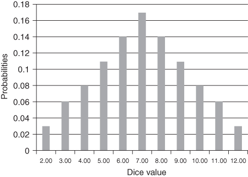
A discrete distribution is just as it sounds, the values of the variable are discrete. For instance, there is no such thing as a 7.5 on a pair of dice. It is a value of 7 or 8. Same as with the probabilities of heads or tails on a coin, they are discrete values.

Another example of a discrete distribution would be the probabilities associated with a certain type of car being in a wreck. These are discrete numbers associated with a certain type of vehicle. Common types of discrete variables would be the

• number of times an electrical switch is thrown before failure;
• number of cycles of an airplane before failure of a component;
• number of demands on a fire suppression system before failure;
• number of demands on a backup diesel generator before failure.

However, in some cases, depending on the range of values, a discrete type distribution can appear continuous.

The alternative to discrete distributions is continuous distributions. The number of hours drivers operate a vehicle between accidents can range from some fraction of one to thousands of hours. The values of the variable are continuous. Some common types of continuous variables would be the:

• hours of operation of a pump, valve, piping, controller or other mechanical piece of equipment before failure or between repairs;
• hours of operation of an airplane, ship, car, or train between accidents or repairs.

Common types of continuous distributions used for risk assessment are as follows:

• Normal distribution;
• Uniform distribution;
• Chi-square distribution;
• Weibull distribution;
• Poisson distribution;
• Exponential distribution.

Continuous probability distributions possess a probability density function. As discussed above, a continuous random variable is the one which can take a continuous range of values. For example, the time between pump failures can have an infinite number of values; however, it has a probability zero because there are infinitely many other potential values.

The most important continuous probability distribution for risk analysis and reliability engineering is the exponential distribution. The exponential distribution is considered to be memoryless and is, therefore, a good distribution to model the constant hazard rate of a reliability bathtub curve (3).

The expected value or mean of a variable X that is exponentially distributed is

The variance of X is

The median value is

where λ is a rate parameter. When determining failure rates for components the exponential distribution is one of the preferred continuous distributions because an error factor can be calculated. The error factor is the ratio of the ninety-fifth percentile to the median or fiftieth percentile failure rate (4). For example, if the median value for a pump failure is 2E–3 h and the ninety-fifth percentile failure rate is 1.5E–2 the error factor is

Other continuous probability distributions are used in risk assessment, but are much more difficult to apply for most common types of applications. The Weibull distribution is the most widely used continuous distribution used in modeling reliability. In many cases, what appears to be a continuous variable can be converted to a discrete variable and can, therefore, be much more easily dealt with. Run time hours on a pump can be binned into a set of predefined bins, for instance, low, medium, and high. As with any concept, the simpler way information is presented, the more people will understand it and be able to do something with it.