In This Chapter
Writing a Syntax program and saving it to disk
Modifying the menus to run Syntax programs
Understanding some useful Syntax commands
Most Syntax Command programs are short. That's because one command can do so much. This chapter is about the mechanics of writing and running Syntax programs. If you plan to do much processing with SPSS, you'll certainly be doing some things over and over. If you save those procedures in a Syntax command program, you can just run the program instead of stepping through the process again.
To write a new Syntax program, do the following:
From the main menu, choose File
New Syntax.
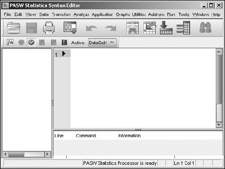
The SPSS Syntax Editor dialog box appears, as shown in Figure 15-1. Use the text area in the upper right of the dialog box to enter the text in the Syntax language. Below the text area is a panel for displaying errors. (The error panel can be resized by dragging the bar at its top.) The panel to the left displays a synopsis of the commands in the program.
Enter the text of the Syntax language in the upper-right panel.
The lines are numbered automatically and can be as long as you need them to be — the window will scroll as necessary.
To execute the program after you write it, choose Run
All.
Syntax programs are tied tightly to the variable definitions in the currently loaded dataset. Syntax programs use the dataset's variable names, often in such a way that the type of the variable can be important. Thus the first instruction in a Syntax program is usually to load the data file.
You can load a file by choosing File
GET FILE='C:Program FilesSPSSInc
  PASWStatistics18SamplesEnglishEmployee data.sav'.
Tip
If you forget the exact form of this command, you can load a file using the menu and see the resulting Syntax command in SPSS Viewer. In fact, running any command by using the menu system causes its Syntax Command sequence to be written to SPSS Viewer.
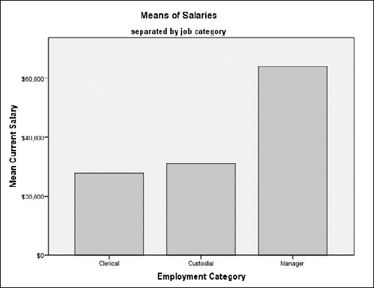
The following is a program with a simple GRAPH command, using the salary and job category information of the loaded data:
GRAPH TITLE = "Means of Salaries"
  /SUBTITLE = "separated by job category"
  /BAR = MEAN(salary) BY jobcat.
The resulting display in SPSS Viewer is shown in Figure 15-2.
To load a Syntax program from disk, choose File
Note
Having the capability to save a copy of your program is important. Whenever you write a Syntax program and think you may want to use it more than once, save it to disk so you can read it into SPSS and run it any time you want.
To save your program, first decide where you want to save it and what you want to call it. Then, in the Syntax Editor dialog box, choose File
Often you'll want to leave your original program as it is and create a new one by making changes to the original. In that case, load the original program from disk and then choose File
Every SPSS menu selection is nothing more than a command to execute a Syntax program. Adding a new item to the menu is a matter of adding a new menu button and assigning a task to it.
You can add new menu selections to customize SPSS and make it easier to do your common tasks. For example, if you're working on a data file and loading it regularly, you could define a new menu button to load the file for you. If you have an analysis or a report-generating program that you run regularly, you could define a menu button that runs it with your set of parameters. Or you could set up a button to export data in your preferred format.
To define terms clearly, a menu consists of the menu bar (the part that's always visible at the top of the window) and its row of pull-down lists. Each list is made up of clickable buttons. Each button can be set to execute a particular Syntax command or to display another list of buttons. You can modify a menu by adding a new pull-down list or by adding a single button to an existing list. You can delete existing menu items, but usually there's no need to do that — your modifications will almost always be for the purpose of adding buttons that perform your own tasks.
The following steps take you through the process of adding a new pull-down list with one button. The button executes the Syntax program named loadfile.sps, which is a program consisting of one GET statement to load a file:
Create
loadfile.sps.Write and save a Syntax program that loads a SPSS data file. This example uses the one-line program (described earlier in this chapter) that uses the
GETcommand to loadEmployee data.sav.Choose View
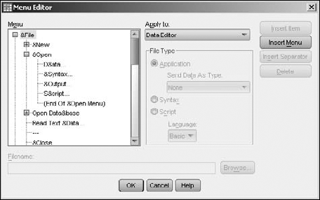
Menu Editor.The dialog box shown in Figure 15-3 appears. You can make this menu choice from any system menu — the main SPSS dialog window, SPSS Viewer, or even Syntax Editor. Any menu can be modified through this dialog box.
In the Apply To pull-down list, select Data Editor.
This is where you choose which menu you're going to modify. The other choices are View and Syntax. Each time you choose a different menu, the buttons that are already defined for that menu show up in the Menu list on the left.
In the list of names in the Menu box, click the plus sign next to &Open.
The list expands to display the items already defined: D&ata, &Syntax, &Output, and S&cript. This followed by an (End Of &Open Menu) notation. The ampersand (&) in the name specifies the following letter to be the shortcut key that activates the menu item. In this example the shortcut letters are A, S, O, and C, You can include an ampersand in the name you add, if you want.
Warning
If you use an ampersand to specify the same letter as a shortcut for more than one menu selection, SPSS will use one and ignore the other — which is probably not what you intended.
Select End Of &Open Menu.
The selection becomes highlighted. Whenever an item is added to the menu, it is added immediately before the selected item. (The End entry is included in the list only so the last position can be selected.)
Click the Insert Item button.
A new menu button with the name New Menu Item appears.
Type the name MyFile and press the Enter key.
The text you type replaces the name of the selected menu item.
In the File Type area, select Syntax.
You can associate the new menu selection with another application or a script if you like; in this example, the new menu selection executes a Syntax program.
Click the Browse button and locate the Syntax program file.
Clicking the button opens a browse window. Locate the directory containing the file
loadfile.sps. To make the filename appear, you may need to choose Syntax Files (*.sps) in the Files Of Type pull-down list at the bottom of the dialog box.Click the OK button.
The Open menu of the main window of SPSS has been modified by the addition of MyFile, as shown in Figure 15-4.
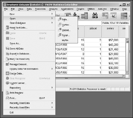
If you want to add this same option to the menus of other dialog boxes in SPSS, you have to follow the same procedure for each one. Adding a menu item takes only a small amount of work and can prevent many repeated steps. For example, if you're in the process of entering and correcting data, a simple menu item to load the file would keep you from hunting for the file every time you need to load it. Also, if you have a group of analyses that you run repeatedly, you could include them all in one Syntax program and have them all run for you at the click of a button. The program could be made to load the file at its startup, so one click of a button is all you need to do all that work.
There are lots of Syntax commands, and they all have lots of options. If you have something you want to do, and you want to find the Syntax command to do it, you have three basic approaches.
One way is to use the menu system to command SPSS to do whatever it is you would like it to do. In SPSS Viewer, you will be able to see the text of the Syntax commands that generated the output. Highlight that text, choose Edit
Another way to find commands is to select Help
A third approach is to select Help
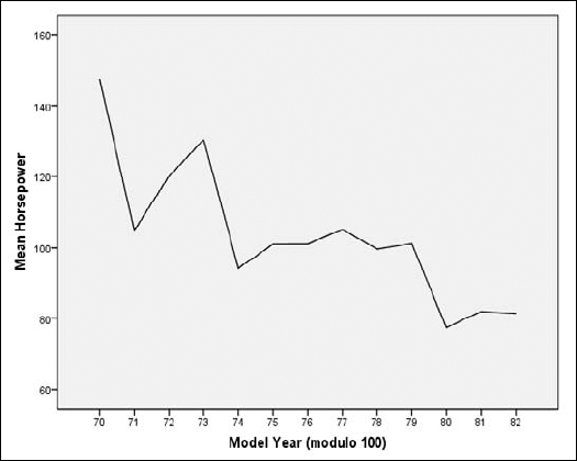
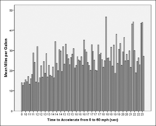
You can write a Syntax program to do more than one thing. All the commands in such a script are executed one after the other. And because one Syntax command can do quite a bit, you don't have to write much of a program to do lots of processing. For example, the following four-line program named makeplot.sps performs four separate tasks:
GET FILE='C:Program FilesSPSSIncPASWStatistics18
  SamplesEnglishCars.sav'.
DATASET NAME DataSet1 WINDOW=FRONT.
GRAPH LINE=MEAN (HORSE) BY YEAR.
GRAPH BAR=MEAN (MPG) BY ACCEL.
The first two lines load the SPSS data file named Cars.sav. The third line renames the dataset to DataSet1 and brings the window displaying it to the front. As a result, if data has already been loaded and named DataSet1, this new file assumes the name (the other will be closed). The last two lines draw graphs — one line graph and one bar graph, as shown in Figure 15-5 and 15-6.
Note how variable references are made on the GRAPH commands. Referring to a variable by its name specifies that all its values be used; using the word MEAN before the variable name in parentheses specifies that the mean of the variable's values be used. These commands are simple but the actions are complex.
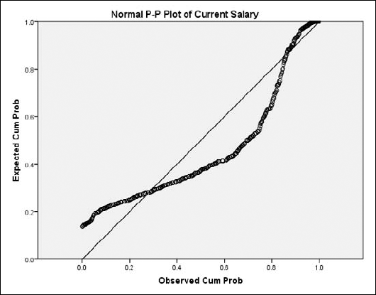
The Syntax language contains the PPLOT command, which you can use to generate either of these types of plots:
The following program, named makeplot2.sps, contains commands to produce both.
GET FILE='C:Program FilesSPSSIncPASWStatistics18
  SamplesEnglishEmployee data.sav'.
DATASET NAME DataSet1 WINDOW=FRONT.
PPLOT SALARY /TYPE=Q-Q.
PPLOT SALARY /TYPE=P-P.
This program loads the dataset and then produces a plot of each type. The q-q plot is displayed in Figure 15-7.
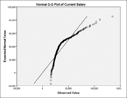
Figure 15-8 displays the p-p plot produced from the program.
Figures 15-7 and 15-8 don't represent all the output you get from the PPLOT command. In particular, a detrended plot (a plot in which the actual values are plotted against deviations of the expected values) is also produced.
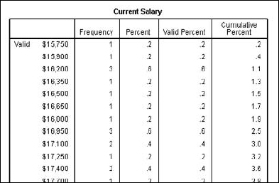
In this section we look at a program that loads a data file and counts the repetition of values in a certain variable. The program counts repetitions for all cases in a file, splits the file, and takes a count for each portion. The program is named splitfile.sps:
GET FILE='C:Program FilesSPSSIncPASWStatistics18
  SamplesEnglishEmployee data.sav'.
FREQUENCIES SALARY.
SORT CASES BY GENDER.
SPLIT FILE BY GENDER.
FREQUENCIES SALARY.
The first line of the program uses the GET command to load the file. The second line uses the FREQUENCIES command to generate the counts and percentages for the salary values. The top section of the table produced from this command is shown in Figure 15-9. As you can see, the table that the program generated includes five columns. A salary value is shown in the first column; a count of the total number of occurrences of the value appears in the second column. The Percent column holds the percent of the total number of cases (excluding cases with missing values in any variable) that contain this particular salary value. The Valid Percent column holds the percent of the total number of cases (including those with missing values in other variables) that contain this particular value. The Cumulative Percent is the number of cases with salaries less than or equal to the salary shown in the first column. For this example, the values displayed as Percent and Valid Percent are the same because no cases in the displayed portion contain a missing value for any variable.
Then comes the split. The program that sorts cases uses the SORT command to do the split. You must sort a dataset using the same variable as the key that's about to be used to split a file; variables of like values must be all together for the split to work properly. In this example, the SORT command groups all the female cases before the male cases.
The SPLIT command logically inserts a divider at each point where the value of the named variable changes. In this example, the value f is used for female and the value m for male, so a logical divider is placed between them. The divider is logical because the split refers only to the memory-resident form of the data — the split does not survive the data being written to a file.
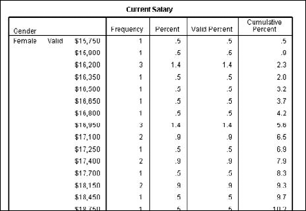
The last line of the program builds a new set of counts and percentages, but this time the data is divided by gender, so the table is generated in two parts. The upper part of the table is shown in Figure 15-10. The headings of the table have the same meanings they had before, but you can see that the top of the table contains the numbers for the female cases. The bottom portion contains data from males. If the SPLIT command had used a variable with more values, the cases would have been split into more parts.
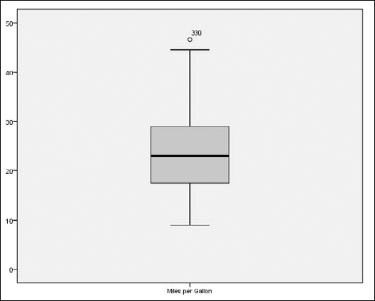
The EXAMINE command in the Syntax language may be the quickest way to look at data. For example, with the system data file named Cars.sav loaded into SPSS, a two-word Syntax program produces a graph of a variable. The two-word program is as follows:
EXAMINE MPG.
This command results in the box plot shown in Figure 15-11, which graphically displays the mean, the standard deviation, and the extreme values.
But that's not the only way EXAMINE can show you data. You can include more than one variable, or you can change the plot style to a histogram. The following command generates more than one histogram:
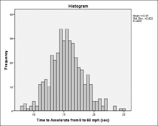
EXAMINE ACCEL, HORSE /PLOT=HISTOGRAM.
This command produces a histogram for each of the two named variables. The histogram representing the acceleration values (ACCEL) is shown in Figure 15-12.