7. Working with Groups of Rows
The queries you have seen so far in this book for the most part operate on one row at a time. However, SQL also includes a variety of keywords and functions that work on groups of rows—either an entire table or a subset of a table. In this chapter you will read about what you can do to and with grouped data.
Note: Many of the functions that you will be reading about in this chapter are often referred to as SQL's OLAP (Online Analytical Processing) functions.
Set Functions
The basic SQL set, or aggregate, functions (summarized in Table 7-1) compute a variety of measures based on values in a column in multiple rows. The result of using one of these set functions is a computed column that appears only in a result table.
The basic syntax for a set function is
Function_name (input_argument)
You place the function call following SELECT, just as you would an arithmetic calculation. What you use for an input argument depends on which function you are using.
Note: For the most part, you can count on a SQL DBMS supporting COUNT, SUM, AVG, MIN, and MAX. In addition, many DBMSs provide additional aggregate functions for measures such as standard deviation and variance. Consult the DBMSs documentation for details.
COUNT
The COUNT function is somewhat different from other SQL set functions in that instead of making computations based on data values, it counts the number of rows in a table. To use it, you place COUNT (*) in your query. COUNT's input argument is always an asterisk:
SELECT COUNT (*)
FROM volume;
The response appears as
count
- - - - - - -
71
To count a subset of the rows in a table, you can apply a WHERE predicate:
SELECT COUNT (*)
FROM volume
WHERE isbn = ‘978-1-11111-141-1’;
The result—
Count
- - - - - - -
7
—tells you that the store has sold or has in stock seven books with an ISBN of 978-1-11111-141-1. It does not tell you how many copies of the book are in stock or how many were purchased during any given sale because the query is simply counting the number of rows in which the ISBN appears. It does not take into account data in any other column.
Alternatively, the store could determine the number distinct items contained in a specific order with a query like
SELECT COUNT (*)
FROM volume
WHERE sale_id = 6;
When you use * as an input parameter to the COUNT function, the DBMS includes all rows. However, if you wish to exclude rows that have nulls in a particular column, you can use the name of the column as an input parameter. To find out how many volumes are currently in stock, the rare book store could use
SELECT COUNT (selling_price)
FROM volume;
If every row in the table has a value in the selling_date column, then COUNT (selling_date) is the same as COUNT (*). However, if any rows contain null, then the count will exclude those rows. There are 71 rows in the volume table. However, the count returns a value of 43, indicating that 43 volumes have not been sold and therefore are in stock.
You can also use COUNT to determine how many unique values appear in any given column by placing the keyword DISTINCT in front of the column name used as an input parameter. For example, to find out how many different books appear in the volume table, the rare book store would use
SELECT COUNT (DISTINCT isbn)
FROM volume;
The result—27—is the number of unique ISBNs in the table.
SUM
If someone at the rare book store wanted to know the total amount of an order so that value could be inserted into the sale table, then the easiest way to obtain this value is to add up the values in the selling_price column:
The result appears as
sum
- - - - - - - -
505.00
In the preceding example, the input argument to the SUM function was a single column. However, it can also be an arithmetic operation. For example, to find the total of a sale if the books are discounted 15 percent, the rare book store could use the following query:
SELECT SUM (selling_price * .85)
FROM volume
WHERE sale_id = 6;
The result—
sum
- - - - - - - - - -
429.2500
—is the total of the multiplication of the selling price times the selling percentage after the discount.
If we needed to add tax to a sale, a query could then multiply the result of the SUM by the tax rate:
SELECT SUM (selling_price * .85) * 1.0725
FROM volume
WEHRE sale_id = 6;
producing a final result of 429.2500.
Note: Rows that contain nulls in any column involved in a SUM are excluded from the computation.
AVG
The AVG function computes the average value in a column. For example, to find the average price of a book, someone at the rare book store could use a query like
SELECT AVG (selling_price)
FROM volume;
The result is 68.2313953488372093 (approximately $68.23).
Note: Rows that contain nulls in any column involved in an AVG are excluded from the computation.
MIN and MAX
The MIN and MAX functions return the minimum and maximum values in a column or expression. For example, to see the maximum price of a book, someone at the rare book store could use a query like
SELECT MAX (selling_price)
FROM volume;
The result is a single value: $205.00.
The MIN and MAX functions are not restricted to columns or expression that return numeric values. If someone at the rare book store wanted to seethe latest date on which a sale had occurred, then
SELECT MAX (sale_date)
FROM volume;
returns the chronologically latest date (in our particular sample data, 01-Sep-13).
By the same token, if you use
SELECT MIN (last_name)
FROM customer;
you will receive the alphabetically first customer last name (Brown).
Set Functions in Predicates
Set functions can also be used in WHERE predicates to generate values against which stored data can be compared. Assume, for example, that someone at the rare book store wants to see the titles and cost of all books that were sold that cost more than the average cost of a book.
The strategy for preparing this query is to use a subquery that returns the average cost of a sold book and to compare the cost of each book in the volume table to that average:
SELECT title, selling_price
FROM work, book, volume
WHERE work.work_numb = book.work_numb
AND book.isbn = volume.isbn
AND selling_price > (SELECT AVG (selling_price) FROM volume);
Although it would seem logical that the DBMS would calculate the average once and use the result of that single computation to compare to rows in the volume, that's not what happens. This is actually an uncorrelated subquery; the DBMS recalculates the average for every row in volume. As a result, a query of this type will perform relatively slowly on large amounts of data. You can find the result in Figure 7-1.
 |
| Figure 7-1 Output of a query that uses a set function in a subquery |
Changing Data Types: CAST
One of the problems with the output of the SUM and AVG functions that you saw in the preceding section of this chapter is that they give you no control over the precision (number of places to the right of the decimal point) of the output. One way to solve that problem is to change the data type of the result to something that has the number of decimal places you want using the CAST function.
CAST requires that you know a little something about SQL data types. Although we will cover them in depth in Chapter 8, a brief summary can be found in Table 7-2.
To restrict the output of the average price of books to a precision of 2, you could then use
CAST (AVG (selling_price) AS DECIMAL (10,2))
and incorporate it into a query using
SELECT CAST (AVG (selling_price) AS DECIMAL (10,2))
FROM volume;
The preceding specifies that the result should be displayed as a decimal number with a maximum of 10 characters (including the decimal point) with two digits to the right of the decimal point. The result is 68.23, a more meaningful currency value than the original 68.2313953488372093.
CAST also can be used, for example, to convert a string of characters into a date. The expression
CAST ('10-Aug-2013' AS DATE)
returns a datetime value.
Valid conversions for commonly used data types are represented by the light gray boxes in Table 7-3. Those conversions that may be possible if certain conditions are met are represented by the dark gray boxes. In particular, if you are attempting to convert a character string into a shorter string, the result will be truncated.
Grouping Queries
SQL can group rows based on matching values in specified columns and computer summary measures for each group. When these grouping queries are combined with the set functions that you saw earlier in this chapter, SQL can provide simple reports without requiring any special programming.
Forming Groups
To form a group, you add a GROUP BY clause to a SELECT statement, followed by the columns whose values are to be used to form the groups. All rows whose values match on those columns will be placed in the same group.
For example, if someone at the rare book store wants to see how many copies of each book edition have been sold, he or she can use a query like
SELECT isbn, COUNT(*)
FROM volume
GROUP BY isbn
ORDER BY isbn;
The query forms groups by matching ISBNs. It displays the ISBN and the number of rows in each group (see Figure 7-2).
 |
| Figure 7-2 Counting the members of a group |
There is a major restriction that you must observe with a grouping query: You can display values only from columns that are used to form the groups. As an example, assume that someone at the rare book store wants to see the number of copies of each title that have been sold. A working query could be written
The result appears in Figure 7-3. The problem with this approach is that titles may duplicate. Therefore, it would be better to group by the work number. However, given the restriction as to what can be displayed, you wouldn't be able to display the title.
 |
| Figure 7-3 Grouping rows by book title |
The solution is to make the DBMS do a bit of extra work: Group by both the work number and the title. The DBMS will then form groups that have the same values in both columns. There is only one title per work number, so the result will be the same as that in Figure 7-3 if there are no duplicated titles. We therefore gain the ability to display the title when grouping by the work number. The query could be written
SELECT work.work_numb title, COUNT (*)
FROM volume, book, work
WHERE volume.isbn = book.isbn
AND book.work_numb = work.work_numb
GROUP BY work_numb, title
ORDER BY title;
As you can see in Figure 7-4, the major difference between the two results is the appearance of the work number column.
 |
| Figure 7-4 Grouped output using two grouping columns |
You can use any of the set functions in a grouping query. For example, someone at the rare book store could generate the total cost of all sales with
SELECT sale_id, SUM (selling_price)
FROM volume
GROUP BY sale_id;
The result can be seen in Figure 7-5. Notice that the last line of the result has nulls for both output values. This occurs because those volumes that haven't been sold have null for the sale ID and selling price. If you wanted to clean up the output, removing rows with nulls, you could add a WHERE clause:
SELECT sale_id, SUM (selling_price)
FROM volume
WHERE NOT (sale_id IS NULL)
GROUP BY sale_id;
 |
| Figure 7-5 The result of using a set function in a grouping query |
Including the title as part of the GROUP BY clause was a trick to allow us to display the title in the result. However, more commonly we use multiple columns to created nested groups. For example, if someone at the rare book store wanted to see the total cost of purchases made by each customer per day, the query could be written
SELECT customer.customer_numb, sale_date, SUM (selling_price)
FROM customer, sale, volume
WHERE customer.customer_numb = sale.customer_numb
AND sale.sale_id = volume.sale_id
GROUP BY customer.customer_numb, sale_date;
Because the customer_numb column is listed first in the GROUP BY clause, its values are used to create the outer groupings. The DBMS then groups orders by date within customer numbers. The default output (see Figure 7-6) is somewhat hard to interpret because the outer groupings are not in order. However, if you add an ORDER BY clause to sort the output by customer number, you can see the ordering by date within each customer (see Figure 7-7).
 |
| Figure 7-6 Group by two columns (default row order) |
 |
| Figure 7-7 Grouping by two columns (rows sorted by outer grouping column) |
Restricting Groups
The grouping queries you have seen to this point include all the rows in the table. However, you can restrict the rows that are included in grouped output using one of two strategies:
◊ Restrict the rows before groups are formed.
◊ Allow all groups to be formed and then restrict the groups.
The first strategy is performed with the WHERE clause in the same way we have been restricting rows to this point. The second requires a HAVING clause, which contains a predicate that applies to groups after they are formed.
Assume, for example, that someone at the rare book store wants to see the number of books ordered at each price over $75. One way to write the query is to use a WHERE clause to throw out rows with a selling price less than or equal to $75:
SELECT selling_price, count (*)
FROM volume
WHERE selling_price > 75
GROUP BY selling_price;
Alternatively, you could let the DBMS form the groups and then throw out the groups that have a cost less than or equal to $75 with a HAVING clause:
SELECT selling_price, count (*)
FROM volume
GROUP BY selling_price
HAVING selling_price > 75;
The result in both cases is the same (see Figure 7-8). However, the way in which the query is processing is different.
 |
| Figure 7-8 Restrict groups to volumes that cost more than $75 |
Windowing and Window Functions
Grouping queries have two major drawbacks: They can't show you individual rows at the same time they show you computations made on groups of rows and you can't see data from non-grouping columns unless you resort to the group making trick shown earlier. The more recent versions of the SQL standard (from SQL:2003 onward), however, include a new way to compute aggregate functions yet display the individual rows within each group: windowing. Each window (or partition) is a group of rows that share some criteria, such as a customer number. The window has a frame that “slides” to present to the DBMS the rows that share the same value of the partitioning criteria. Window functions are a special group of functions that can act only on partitions.
Note: By default, a window frame includes all the rows as its partition. However, as you will see shortly, that can be changed.
Let's start with a simple example. Assume that someone at the rare book store wants to see the volumes that were part of each sale as well as the average cost of books for each sale. A grouping query version wouldn't be able to show the individual volumes in a sale nor would it be able to display the ISBN or sale ID unless those two values were added to the GROUP BY clause. However, what if the query were written using windowing—
SELECT sale_id, isbn, CAST (AVG(selling_price)
OVER (PARTITION BY sale_id) as DECIMAL (7.2))
FROM volume
WHERE sale_id IS NOT NULL;
—it would produce the result in Figure 7-9. Notice that the individual volumes from each sale are present and that the rightmost column contains the average cost for the specific sale on which a volume was sold. This mean that the avg column in the result table is the same for all rows that come from a given sale.
 |
| Figure 7-9 Output of a simple query using windowing |
The query itself includes two new keywords: OVER and PARTITION BY. (The CAST is present to limit the display of the average to a normal money display format and therefore isn't part of the windowing expression.) OVER indicates that the rows need to be grouped in some way. PARTITION BY indicates the criteria by which the rows are to be grouped. This particular example computes the average for groups of rows that are separated by their sale ID.
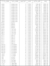
To help us explore more of what windowing can do, we're going to need a sample table with some different types of data. Figure 7-10 (a) shows you a table that describes sales representative and the value of product they have sold in specific quarters. The names of the sales reps are stored in the table labeled (b) in Figure 7-10.
Note: Every windowing query must have an ORDER clause, but you can leave out the PARTITION BY clause—using only OVER ()—if you want all the rows in the table to be in the same partition.
 |
 |
| Figure 7-10 Quarterly sales tables for use in windowing examples |
Ordering the Partitioning
When SQL processes a windowing query, it scans the rows in he order they appear in the table. However, you control the order in which rows are processed by adding an ORDER BY clause to the PARTITION BY expression. As you will see, doing so can alter the result, producing a “running” average or sum.
Consider first a query similar to the first windowing example:
SELECT first_name, last_name, quarter, year, sales_amt, CAST (AVG (sales_amt OVER (PARTITION BY quarterly_sales.sales_id) AS DECIMAL (7,2))
FROM rep_names, quarterly_sales
WHERE rep_names.id = quarterly_sales.id;
As you can see in Figure 7-11, the output is what you would expect: Each line displays the average sales for the given sales representative. The DBMS adds up the sales for all quarters for the salesperson and divides by the number of quarters. However, if we add an ORDER BY clause to force processing in quarter and year order, the results are quite different.
 |
| Figure 7-11 Computing the windowed average without ordering the rows |
The query changes only a bit:
SELECT first_name, last_name, quarter, year, sales_amt, CAST (AVG (sales_amt OVER (PARTITION BY quarterly_sales.sales_id
ORDER BY year, quarter) AS DECIMAL (7,2))
FROM rep_names, quarterly_sales
WHERE rep_names.id = quarterly_sales.id;
However, in this case the ORDER BY clause forces the DBMS to process the rows in year and quarter order. As you can see in Figure 7-12, the average column is now a moving average. What is actually happening is that the window frame is changing in the partition each time a row is scanned. The first row in a partition is averaged by itself. Then the window frame expands to include two rows and both are included in the average. This process repeats until all the rows in the partition have been included in the average. Therefore, each line in the output of this version of the query gives you the average at the end of that quarter rather than for all quarters.
Note: If you replace the AVG in the preceding query with the SUM function, you'll get a running total of the sales made by each sales representative.
 |
| Figure 7-12 Computing the windowed average with row ordering |
If you don't want a running sum or average, you can use a frame clause to change the size of the window (which rows are included). To suppress the cumulative average in Figure 7-12, you would add ROWS BETWEEN UNBOUNDED PRECEDING AND CURRENT ROW following the columns by which the rows within the partition are to be ordered.
Specific Functions
The window functions built into SQL perform actions that are only meaningful on partitions. Many of them include ways to rank data, something that is difficult to do otherwise. They can also number rows and compute distribution percentages. In this section we'll look at some of the specific functions: what they can do for you and how they work.
Note: Depending on your DBMS, you may find additional window functions available, some of which are not part of the SQL standard.
RANK
The RANK function orders and numbers rows in a partition based on the value in a particular column. It has the general format
RANK () OVER (partition_specifications)
For example, if we wanted to see all the quarterly sales data ranked for all the sales representatives, the query could look like the following:
SELECT first_name, last_name quarter, year, sales_amt, RANK () OVER (order by sales_amt desc)
FROM rep_names, quarterly_sales
WHERE rep_names.id = quarterly_sales.id;
The output appears in Figure 7-13. Notice that because there is no PARTITION BY clause in the query, all of the rows in the table are part of a single ranking.
 |
| Figure 7-13 Ranking all quarterly sales |
Alternatively, you could rank each sales representative's sales to identify the quarters in which each representative sold the most. The query would be written
The output can be found in Figure 7-14.
 |
| Figure 7-14 Ranking within partitions |
PERCENT_RANK
Note: When there are duplicate rows, the RANK function includes only one of the duplicates. However, if you want to include the duplicates, use DENSE_RANK instead of RANK.
The PERCENT_RANK function calculates the percentage rank of each value in a partition relative to the other rows in the partition. It works in the same way as RANK but rather than returning a rank as an integer, it returns the percentage point at which a given value occurs in the ranking.
Let's repeat the query used to illustrate RANK, using PERCENT_RANK instead:
SELECT first_name, last_name, quarter, year, sales_amt, PERCENT_RANK () OVER (PARTITION BY quarterly_sales.id ORDER BY sales_amt DESC)
FROM rep_names, quarterly_sales
WHERE rep_names.id = quarterly_sales.id;
ROW_NUMBER
The output can be found in Figure 7-15. As you can see, the result is exactly the same as the RANK result in Figure 7-14, with the exception of the rightmost column, where the integer ranks are replaced by percentage ranks.
 |
| Figure 7-15 Percent ranking within partitions |
The ROW_NUMBER function numbers the rows within a partition. For example, to number the sales representatives in alphabetical name order, the query could be
SELECT first_name, last_name ROW_NUMBER () OVER (ORDER BY last_name, first_name) AS row_numb
FROM rep_names;
As you can see from Figure 7-16, the result includes all 10 sales representatives, numbered and sorted by name (last name as the outer sort).
Given the power and flexibility of SQL's windowing capabilities, is there any time that you should use grouping queries instead? Actually, there just might be. Assume that you want to rank all the sales representatives based on their total sales rather than simply ranking within each person's sales. Probably the easiest way to get that ordered result is to use a query like the following:
SELECT id, SUM (sales_amt)
FROM quarterly_sales
GROUP BY id
ORDER BY SUM (sales_amt) DESC;
You get the following output:
| id | sum |
|---|---|
| 6 | 8027.00 |
| 5 | 7200.00 |
| 2 | 7194.00 |
| 1 | 5570.00 |
| 7 | 4781.00 |
| 3 | 4309.00 |
| 4 | 4177.00 |
| 8 | 4115.00 |
| 10 | 1964.00 |
| 9 | 889.00 |
The highest ranking total sales are at the top of the listing, the lowest ranking sales at the bottom. The output certainly isn't as informative as the windowed output because you can't include the names of the sales representatives, but it does provide the required information.
Yes, you could use a windowing function to generate the same output, but it still needs to include the aggregate function SUM to generate the totals for each sales representative:
It works, but it's more code and the presence of the GROUP BY clause still means that you can't include the names unless they are part of the grouping criteria. Using the GROUP BY and the simple SUM function just seems easier.
Note: The SQL standard allows a named ROW_NUMBER result to be placed in a WHERE clause to restrict the number of rows in a query. However, not all DBMSs allows window functions in WHERE clauses.
 |
| Figure 7-16 Row numbering |
CUME_DIST
When we typically think of a cumulative distribution, we think of something like that in Table 7-5, where the actual data values are gathered into ranges. SQL, however, can't discern the data grouping that we would like and therefore must consider each value (whether it be an individual data row or a row of an aggregate function result) as a line in the distribution.
| Sales amount | Frequency | Cumulative Frequency | Cumulative Percentage |
|---|---|---|---|
| $0–1999 | 2 | 2 | 20 |
| $2000–3999 | 0 | 0 | 20 |
| $4000–5999 | 5 | 7 | 70 |
| $6000–7999 | 2 | 9 | 90 |
| > $8000 | 1 | 10 | 100 |
The CUME_DIST function returns a value between 0 and 1, which when multiplied by 100, gives you a percentage. Each “range” in the distribution, however, is a single value. In other words, the frequency of each group is always 1. As an example, let's create a cumulative frequency distribution of the total sales made by each sales representative. The SQL can be written
SELECT id, SUM (sales_amt), 100 * (CUME_DIST() OVER (ORDER BY SUM (sales_amt))) AS cume_dist
FROM quarterly_sales
GROUP BY id
ORDER BY cume_dist;
As you can see in Figure 7-17, each range is a group of 1.
 |
| Figure 7-17 A SQL-generated cumulative frequency distribution |
NTILE
NTILE breaks a distribution into a specified number of partitions and indicates which rows are part of which group. SQL keeps the numbers of rows in each group as equal as possible. To see how this works, consider the following query:
SELECT id, SUM (sales_amt), NTILE(2)
OVER (ORDER BY SUM (sales_amt) DESC) AS n2, NTILE(3) OVER (ORDER BY SUM (sales_amt DESC) as n3, NTILE(4) OVER (ORDER BY SUM (sales_amt DESC) as n4
FROM quarterly_sales
GROUP BY id;
For the result, see Figure 7-18. The columns labeled n2, n3, and n4 contain the results of the NTILE calls. The highest number in each of those columns corresponds to the number of groups into which the data have been placed, which is the same value used as an argument to the function call.
 |
| Figure 7-18 Using the NTILE function to divide data into groups |
Inverse Distributions: PERCENTILE_CONT and PERCENTILE_DISC
The SQL standard includes two inverse distribution functions—PERCENTILE_CONT and PERCENTILE_DISC—that are most commonly used to compute the median of a distribution. PERCENTILE_CONT assumes that the distribution is continuous and interpolates the median as needed. PERCENTILE_DISC, which assumes a discontinuous distribution, chooses the median from existing data values. Depending on the data themselves, the two functions may return different answers.
The functions have the following general format:
PERCENTILE_cont/disc (0.5)
WITHIN GROUP (optional ordering clause)
OVER (optional partition and ordering clauses)
If you replace the 0.5 following the name of the function with another probability between 0 and 1, you will get the nth percentile. For example, 0.9 returns the 90th percentile. Each function examines the percent rank of the values in a partition until it finds the one that is equal to or greater than whatever fraction you've placed in parentheses.
When used without partitions, each function returns a single value. For example,
SELECT PERCENTILE_CONT (0.5)
WITHIN GROUP (ORDER BY SUM (sales_amt) DESC) AS continuous, PERCENTILE_DISC (0.5)
WITHIN GROUP (ORDER BY SUM (sales_amt DESC) AS discontinuous
FROM quarterly_sales
GROUP BY id;
Given the sales data, both functions return the same value: 1200. (There are 40 values, and the two middle values are 1200. Even with interpolation the continuous median computes to the same answer.)
If we partition the data by sales representative, then we can compute the median for each sales representative:
SELECT first_name, last_name,
PERCENTILE_CONT (0.5) WITHIN GROUP (ORDER BY SUM (sales_amt) DESC) OVER (PARTITION BY id) AS continuous,
PERCENTILE_DISC (0.5) WITHIN GROUP (ORDER BY SUM (sales_amt DESC) OVER (PARTITION BY id) as discontinuous
FROM quarterly_sales JOIN rep_names
GROUP BY id
ORDER BY last_name, first_name;
As you can see in Figure 7-19, the result contains one row for each sales representative, including both medians.
 |
| Figure 7-19 Continuous and discontinuous medians for partitioned data |
..................Content has been hidden....................
You can't read the all page of ebook, please click here login for view all page.