Labeling a set of observations for classification or regression can be a daunting task, especially in the case of a large features set. In some cases, labeled observations are either unavailable or not possible to create. In an attempt to extract some hidden associations or structures from observations, the data scientist relies on unsupervised learning techniques to detect patterns or similarity in data.
The goal of unsupervised learning is to discover patterns of regularities and irregularities in a set of observations. These techniques are also applied in reducing the solution or features space.
There are numerous unsupervised algorithms; some are more appropriate to handle dependent features, while others generate affinity groups in the case of hidden features [4:1]. In this chapter, you will learn three of the most common unsupervised learning algorithms:
- K-means: Clustering observed features
- Expectation-Maximization (EM): Clustering observed and latent features
- Function approximation
Any of these algorithms can be applied to technical analysis or fundamental analysis. Fundamental analyses of financial ratios and technical analyses of price movements are described in the Technical analysis section under Finances 101 in the Appendix . The K-means algorithm is fully implemented in Scala, while the EM and principal components analyses leverage the Apache commons math library.
The chapter concludes with a brief overview of dimension reduction techniques for non-linear models.
Problems involving many features for large datasets become quickly intractable, and it is quite difficult to evaluate the independence between features. Any computation that requires some level of optimization and, at a minimum, the computation of first order derivatives, demands a significant amount of computing power to manipulate high-dimension matrices. As with many engineering fields, a divide and conquer approach to classifying very large datasets is quite appropriate. The objective is to reduce very large sets of observations into a small group of observations that share some common attributes:

Visualization of data clustering
This approach is known as vector quantization. Vector quantization is a method that divides a set of observations into groups of similar sizes. The main benefit of vector quantization is that analysis using a representative of each group is far simpler than an analysis of the entire dataset [4:2].
Clustering, also known as cluster analysis, is a form of vector quantization that relies on a concept of distance or similarity to generate groups known as clusters.
This chapter introduces two of the most commonly applied clustering algorithms:
- K-means, which is used for quantitative types and minimizes the total error (known as the reconstruction error) given the number of clusters and the distance formula.
- Expectation-Maximization (EM), which is a two-step probabilistic approach that maximizes the likelihood estimates of a set of parameters. EM is particularly suitable for handling missing data.
K-means is a popular clustering algorithm that can be implemented either iteratively or recursively. The representative of each cluster is computed as the center of the cluster, known as the centroid. The similarity between observations within a single cluster relies on the concept of distance (or similarity) between observations.
There are many ways to measure the similarity between observations. The most appropriate measure has to be intuitive and avoid computational complexity. This section reviews three similarity measures:
- Manhattan distance
- Euclidean distance
- Normalized inner or dot product
The Manhattan distance is defined by the absolute distance between two variables or vectors {xi} and {yi} of the same size (M1):
The implementation is generic enough to compute the distance between two vectors of elements of different types if an implicit conversion between each of these types to Double values is already defined:
def manhattan[@specialized(Double) T: ToDouble,
             @specialized(Double) U: ToDouble](
    x: Array[T], y: Array[U]): Double = {
 val cu: ToDouble[T] = implicitly[ToDouble[T]]
 val cv: ToDouble[U] = implicitly[ToDouble[U]]
 (x,y).zipped.map{case (u,v
      .Math.abs(cu.apply(u)-cv.apply(v))}.sum
}
The ubiquitous Euclidean distance between two vectors {x i} and {y i} of the same size is defined by the following formula (M2):
def euclidean[@specialized(Double) T: ToDouble,
              @specialized(Double) U: ToDouble](
    x: Array[T], y: Array[U]): Double = {
 val cu: ToDouble[T] = implicitly[ToDouble[T]]
 val cv: ToDouble[U] = implicitlouble[U]]
 Math.sqrt((x,y).zipped.map{case (u,v) =>
       sqr(cu.apply(u)- cv.apply(v)).sum)
}
The normalized inner product or cosine distance between two vectors {xi} and {yi} is defined by the following formula (M3):

In this implementation, the computation of the dot product and the norms for each dataset is done simultaneously using the tuple within the fold method:
def cosine[@specialized(Double) T: ToDouble,
           @specialized(Double) U: ToDouble] (
     x: Array[T],
     y: Array[U]): Double = {

  val cu: ToDouble[T] = implicitly[ToDouble[T]]
  val cv: ToDouble[U] = implicitly[ToDouble[U]]
  val norms = (x,y).zipped.map{ case (u,v) => {
     val wu = cu.apply(u)
     val wv = cv.apply(v)
     Array[Double](wu*wv, wu*wu, wv*wv)
   }}./:(Array.fill(3)(0.0))((s, t) => s ++ t)

  norms(0)/sqrt(norms(1)*norms(2))
}
Tip
Performance of zip and zipped
The scalar product of two vectors is one of the most common operations. It is tempting to implement the dot product using the generic zip method:
def dot(x:Array[Double], y:Array[Double]): Array[Double] = x.zip(y).map{case(x, y) => f(x,y) )A functional alternative is to use the Tuple2.zipped method:
def dot(x:Array[Double], y:Array[Double]): Array[Double] = (x, y).zipped map ( _ * _)
If readability is not a primary concern, you can always implement the dot method with a while loop which prevents you from using the ubiquitous while loop.
The main advantage of the K-means algorithm (and the reason for its popularity) is its simplicity [4:3].

The four steps of the K-means algorithm are:
- Clusters the configuration that is initializing the centroids or means mk of the K clusters.
- Clusters the assignment that is assigning observations to the nearest cluster given the centroids mk.
- Error minimization, that is, computing the total reconstruction error.
- Computes the centroids mk that minimize the total reconstruction error for the current assignment:
- Reassigns the observations, given the new centroids mk.
- Repeats the computation of the total reconstruction error until no observations are reassigned.
- Classification of a new observation by assigning the observation to the closest cluster.
We need to define the components of the K-means in Scala before implementing the algorithm.
Let us create the two main components of the K-means algorithms:
- Clusters of observations
- The implementation of the K-means algorithm
The first step is to define a cluster. A cluster is defined by the following parameters:
- Centroid,
center(line 1) - The indices of the observations that belong to this cluster,
members(line 2):class Cluster[T: ToDouble](val center: Array[Double]) { //1 type DistanceFunc[T] = (Array[Double],Array[T]) => Double val members = new ListBuffer[Int] //2 def moveCenter(xt: Vector[Array[T]]): Cluster[T] ... }
The cluster is responsible for managing its members (data points) at any point of the iterative computation of the K-means. It is assumed that a cluster will never contain the same data points twice. The two key methods in the class Cluster are:
moveCenter: Re-computes the centroid of a clusterstdDev: Computes the standard deviation of the distance between all the observation members and the centroid
The constructor of the Cluster class is implemented by the apply method in the companion object (refer to the Class constructors template
section under Source code consideration in the Appendix):
def apply[T: ToDouble](
    center: Array[Double]
  ): Cluster[T] new Cluster[T](center)
}
Let us look at the moveCenter method. It creates a new cluster from the existing members with a new centroid. The computation of the values of the centroid requires the transposition of the matrix of observations by features into a matrix of features by observations (line 3). The new centroid is computed by normalizing the sum of each feature across all the observations by the number of data points (line 4):
def moveCenter(xt: Vector[Array[T]])(
  implicit m: Manifest[T], num: Numeric[T]
): Cluster[T] = {
  val s = transpose(members.map(xt(_)).toList).map(_.sum) //3
  Cluster[T](
    s.map(implicitly[ToDouble[T]].apply(_y(_)/ members.size)) //4
}
The stdDev method computes the standard deviation of all the observations contained in the cluster relative to its center. The distance between each member and the centroid is extracted through a map invocation (line 5). It is then loaded into a statistics instance to compute the standard deviation (line 6). The function to compute the distance between the center and an observation is an argument of the method. The default distance is Euclidean:
def stdDev(xt: Vector[Array[T]],
           distance: DistanceFunc
): Double = {
  val ts = members.map(xt( _)).map(distance(center,_))//5
  Stats[Double](ts).stdDev  //6
}
Note
Cluster selection
There are different ways to select the most appropriate cluster when reassigning an observation (updating its membership). In this implementation, we select the cluster with the larger spread or lowest density. An alternative is to select the cluster with the largest membership.
The initialization of the cluster centroids is important to ensure fast convergence of K-means. Solutions range from the simple random generation of centroids to the application of genetic algorithms to evaluate the fitness of centroid candidates. We selected an efficient and fast initialization algorithm developed by M Agha and W Ashour [4:4].
The steps of the initialization are as follows:
- Compute the standard deviation of the set of observations.
- Compute the index of the feature {xk,0, xk,1 … xk,n} with the maximum standard deviation.
- Rank the observations by their increasing value of standard deviation for the dimension k.
- Divide the ranked observations set equally into K sets {Sm}.
- Find the median values size(Sm)/2.
- Use the resulting observations as initial centroids.
Let's deconstruct the implementation of the Agha-Ashour algorithm in the method initialize:
type U = Vector[Array[T]]
type V = KmeansModel[T]

def initialize(xt: U): V = {
  val stats = statistics(xt) //7
     val mxSDevDim = stats.indices.maxBy(stats( _ ).stdDev )//8
  val rankedObs = xt.zipWithIndex
      .map{ case (x, n) =>
          (implicitly[ToDouble[T]].apply(x(mxSDevDim )), n)
      }.sortBy(_._1)  //9

  val halfSegSize = ((rankedObs.size>>1)/config.K)
                      .floor.toInt //10
  val centroids = rankedObs
     .filter( isContained( _, halfSegSize, rankedObs.size) )
     .map{case(x, n) => xt(n)} //11

  centroids.aggregate(List[Cluster[T]]())((xs, s) => {
     val c = s.map(implicitly[ToDouble[T]].apply(_))
     Cluster[T](c) :: s, _ ::: _)  //12
  }
}
The statistics method on time series of type Vector[Array[T]] is defined in the Time Series section of Chapter 3,
Data Pre-processing (line 7). The dimension (or feature) with the maximum variance or standard deviation mxSDevDim is computed by using the method maxBy on a Stats instance (line 8). Then the observations are ranked by the increasing value of the standard deviation, rankedObs (line 9).
The ordered sequence of observations is then broken into xt.size/config.K segments (line 10) and the indices of the centroids are selected as the mid-point (or median) observations of those segments using the filtering condition isContained (line 11):
def isContained(t: (T,Int), hSz: Int, dim: Int): Boolean =
    (t._2 % hSz == 0) && (t._2 %(hSz<<1) != 0)
Finally, the list of clusters is generated using an aggregate call on the set of centroids (line 12).
The second step in the K-means algorithm is the assignment of the observations to the clusters for which the centroids have been initialized in step 1. This feat is accomplished by the private method, assignToClusters:
def assignToClusters(
    xt: U,
    clusters: V,
 members: Array[Int]): Int =  {

  xt.zipWithIndex.filter{ case(x, n) => {  //13
    val nearestCluster = getNearestCluster(clusters, x) //14
    val reassigned = nearestCluster != members(n)
    clusters(nearestCluster) += n //15
    members(n) = nearestC/16
    reassigned
  }}.size
}
The core of the assignment of observations to each cluster is the filter on the time series (line 13). The filter computes the index of the closest cluster and checks if the observation is to be reassigned (line 14). The observation at index n is added to the nearest cluster, clusters(nearestCluster) (line 15). The current membership of the observations is then updated (line 16).
The cluster closest to an observation data is computed by the private method getNearestCluster as follows:
def getNearestCluster(model: V, x: Array[T]): Int =
  model.zipWithIndex./:((Double.MaxValue, 0)){
    case (p, (c, n) ) => {
     val measure = distance(c.center, x) //17
     if(measure < p._1 (measure, n)  else p
  }}._2
A fold is used to extract from the list of clusters the cluster that is closest to the observation x using the distance metric defined in the K-means constructor (line 17).
As with other data processing units, the extraction of K-means clusters is encapsulated in a data transformation so clustering can be integrated into a workflow using the composition of mixins described in the Composing mixins to build workflow section in Chapter 2, Data Pipelines.
Tip
K-means algorithm exit condition
In some rare instances, the algorithm may reassign the same few observations between clusters, preventing its convergence toward a solution in a reasonable time. Therefore, it is recommended to add a maximum number of iterations as an exit condition. If K-means does not converge with the maximum number of iterations, then the cluster centroids need to be re-initialized and the iterative (or recursive) execution needs to be re-started.
The transformation |> requires the computation of the standard deviation of the distance of the observations related to the centroid c and is computed in the method stdDev:
def stdDev[T: ToDouble](
    model: KMeansModel[T],
    xt: Vector[Array[T]],
    dance: DistanceFunc[T]): DblVector =
model.map( _.stdDev(xt, distance)).toVectorThe clusters are initialized with a predefined set of observations as their members. The algorithm updates the membership of each cluster by minimizing the total reconstruction error. There are two effective strategies to execute the K-means algorithm:
- Tail recursive execution
- Iterative execution
Let us declare the K-means algorithm class, KMeans, with its public methods. KMeans implements a data transformation, ITransform, using an implicit model extracted from a training set and described in the Monadic data transformation
section of Chapter 2, Data Pipeline (line 18). The configuration of type KMeansConfig consists of the tuple (K, maxIters), with K being the number of clusters and maxIters the maximum number of iterations allowed for the convergence of the algorithm:
case class KMeansConfal K: Int, maxIters: Int)
The KMeans class takes three arguments:
Config: The configuration for execution of the algorithmDistance: The function to compute the distance between any observation and a cluster centroidXt: The training set
The implicit conversion of type T to a Double is implemented as a view bound. The instantiation of the KMeans class initializes type V of the output from K-means as Cluster[T] (line 20). The instance num of the class Numeric has to be passed implicitly as a class parameter because it is required by the sortWith invocation in initialize, the maxBy method, and the Cluster.moveCenter method (line 19). The Manifest is required to preserve the type erasure for Array[T] in the JVM:
class KMeans[@specialized(Double) T: ToDouble](
    config: KMeansConfig,  //18
    distance: DistanceFunc[T],
    xt: Vector[Array[T]]
)(implicit m: Manifest[T], num: Numeric[T]) //19
extends ITransform[Array[T], Cluster[T]) with Monitor[T] {

  type V = Cluster[T] //20
  val model: Option[KMeansModel[T]] = train
  def train: Option[KMeansModel[T]] = ???
  override def |> : PartialFunction[Array[T], Try[V]]
  ...
}
The model of type KMeansModel is defined as the list of clusters extracted through training.
The transformation or clustering function is implemented by the training method train that creates a partial function with Vector[Array[T]] as input and KMeansModel[T] as output:
def train: Option[KMeansModel[T]] = Try {
         // STEP 1
  val clusters = initialize(xt) //21
  if( clusters.isEmpty)  /* ...  */
  else {
         // STEP 2
    val members = Array.fill(xt.size)(0)
    assignToClusters(xt, clusters, members) //22
    var iters = 0
    if(iters >= config.maxIters) throw new IllegalStateException()
         // STEP 3
    update(clusters, xt, members)  //23
  }
} match { /* …*/
}
The K-means training algorithm is implemented through the following three steps:
- Initialize the clusters centroid using the method
initialize(line 11) - Assign observations to each of the clusters through the method
assignToClusters(line 22) - Re-compute the total error reconstruction using the recursive method
update(line 23)
The computation of the total error reconstruction is implemented as a tail recursive method, update:
@tailrec
def update(clusters: KMeansModel[T],
           xt: U,
           members: Array[Int]): KMeansModel[T] = {  //24

  val newClusters = clusters.map(c => {
     if( c.size > 0) c.moveCenter(xt) //25
     else clusters.filter( _.size >0)
          .maxBy(_.stdDev(xt, distance)) //26
  })
  iters += 1
  if( iters >= config.maxIters ||       //27
      assignToClusters(xt, newClusters, members) ==0)
    newClusters
  else update(newClusters, xt, membership)   //28
}
The recursion takes three arguments (line 24):
- The current list of
clustersthat updated during the recursion - The input time series,
xt - The indices of membership to the clusters,
members
A new list of clusters, newClusters, is computed by either recalculating each centroid if the cluster is not empty (line 25) or evaluating the standard deviation of the distance of each observation relative to each centroid otherwise (line 26). The execution exits when either the maximum number of recursive calls, maxIters, is reached or there are no more observations reassigned to a different cluster (line 27). Otherwise, the method invokes itself with an updated list of clusters (line 28).
The implementation of iterative execution is presented for informational purposes. It follows the same sequence of calls as with the recursive implementation. The new clusters are computed (line 29) and the execution exits when either the maximum number of allowed iterations is reached (line 30) or there are no more observations reassigned to a different cluster (line 31):
val members = Array.fill(xt.size)(0)
assignToClusters(xt, clusters, members)
var newClusters = List.empty[Cluster[T]]

(0 until maxIters).find( _ => {  //29
  newClusters = clusters.map( c => {   //30
    if( c.size > 0)  c.moveCenter(xt)
    else clusters.filter( _.size > 0)
                 .maxBy( _.stdDev(xt, distance) )
  })
  assignToClusters(xt, newClusters, members) > 0  //31
}).map(_ => newClusters)
The density of the clusters is computed in the KMeans class as follows:
def density: Option[DblVec] = model.map( _.map(c =>
c.getMembers.map(xt(_)).map( distance(c.center, _))).sum)The objective of the classification is to assign an observation to a cluster with the closest centroid:
override def |> : PartialFunction[Array[T], Try[V]] = {
  case x: Array[T] if( x.length == dimension(xt) &&
                      model.isDefined ) =>
  Try (model.map( _.minBy(c => distance(c.center,x))).get )
}
The most appropriate cluster is computed by selecting the cluster c whose center is the closest to the observation x using the minBy higher order method.
A model with a significant number of features (high dimension) requires a larger number of observations in order to extract relevant and reliable clusters. K-means clustering for very small datasets < 50 produces models with high bias and a limited number of clusters, which are affected by the order of observations [4:5]. I have been using the following simple empirical rule of thumb for a training set of size n, expected K clusters, and N features: n < K.N:
Whichever empirical rule you follow, such a restriction is an issue particularly for analyzing stocks using historical quotes. Let us consider our examples of using technical analysis to categorize stocks according to their price behavior over a period of one year (or approximatively 250 trading days). The dimension of the problem is 250 (250 daily closing prices). The number of stocks (observations) would have exceeded several hundred!

Price model for K-means clustering
There are options to get around this limitation and shrink the numbers of observations; among them are:
- Sampling the trading data without losing a significant amount of information from the raw data, assuming the distribution of observations follows a known probability density function.
- Smoothing the data to remove the noise, as seen in Chapter 3, Data Pre-processing, assuming the noise is Gaussian. In our test, a smoothing technique will remove the price outliers for each stock and therefore reduce the number of features (trading sessions). This approach differs from the first (sampling) technique because it does not require that the dataset follow a known density function. On the other hand, the reduction of features could be less significant.
These approaches are workaround solutions at best, used for the sake of this tutorial. You need to consider the quality of your data before applying these techniques to actual commercial applications. The principal component analysis introduced in the last paragraph is one of the reliable dimensions reduction techniques.
The objective is to extract clusters from a set of stocks' price actions during a period between January 1 and December 31, 2013 as features. For this test, 127 stocks are randomly selected from the S&P 500 list. The following chart visualizes the behavior of the normalized price of a subset of these 127 stocks:

Price action of a basket of stocks used in K-means clustering
The key is to select the appropriate features prior to clustering and the time window to operate on. It would make sense to consider the entire historical price over the 252 trading days as a feature. However, the number of observations (stocks) is too limited to use the entire price range. The observations are the stock closing price for each trading session between the 80th to the 130th trading day. The adjusted daily closing prices are normalized using their respective minimum and maximum values.
First let us create a simple method to compute the density of the clusters:
val MAX_ITERS = 150 def getDensity( K: Int, obs: Vector[Array[Double]]): DblVec = KMeans[Double](KMeansConfig(K, MAX_ITERS)) .density.getOrElse(Vector.empty[sity.get //ethoddensity getDensityinvokes theKMeans.densitydescribed in Step 3. Let us load the data from csv files using theDataSourceclass described in the Data extraction section under Source code consideration in the Appendix: type INPUT = Array[String] => Double val START_INDEX = 80; val NUM_SAMPLES = 50 //33 val extractor = adjClose :: List[INPUT]() //34 val symbolFiles = DataSource.listSymbolFiles(path) //35 for { prices <- getPrices //36 values <- Try( getPricesRange(prices) ) //37 stdDev <- Try( ks.map(getDensity(_, values.toVector))) //38 pfnKmeans <- Try { //39 KMeans[Double](KMeansConfig(5, MAX_ITERS),values) |> } if(pfnKmeans.isDefined) predict <- pfnKmeans(values.head) //40 } yield { val results = s"""Daily prices ${prices.size} stocks") | Clusters density ${stdDev.mkString(", ")}""" .stripMargin show(results) }
As mentioned earlier, the cluster analysis applies to the closing price in the range between the 80th and 130th trading day (line 33). The function extractor retrieves the adjusted closing price for a stock from the Yahoo financials pages YahooFinancials (line 34). The list of stock tickers (or symbols) is extracted as the list of CSV filenames located in the path (line 35). For instance, the ticker symbol for General Electric Corp. is GE and the data is located in GE.csv.
The execution extracts 50 daily prices using DataSource and then filters out the incorrectly formatted data using a filter (line 36):
type XVSeriesSet = Array[Vector[Array[Double]]]

def getPrices: Try[XVSeriesSet] = Try {
  symbolFiles.map( DataSource(_, path) |> extractor )
             .filter( _.isSuccess ).map( _.get)
}
The historical stock prices for the trading session between the 80th and 130th days are generated by the getPricesRange closure (line 37):
def getPricesRange(prices: XVSeriesSet) =
   prices.view.map(_.head.toArray)
        .map( _.drop(START_INDEX).take(NUM_SAMPLES))
It computes the density of the clusters by invoking the method density for each values ks of the number of clusters (line 38).
The partial classification function, pfnKmeans, is created for a five-cluster KMeans (line 39) and is then used to classify one of the observation (line 40).
The first test run is executed with K=3 clusters. The mean (or centroid) vector for each cluster is plotted:
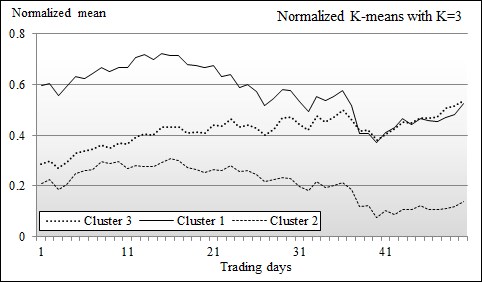
Chart of means of clusters using K-means K=3
The means vectors of the three clusters are quite distinctive. The top and bottom means 1 and 2 in the chart have the respective standard deviation of 0.34 and 0.27 and share a very similar pattern. The difference between the elements of the 1 and 2 clusters' mean vectors is almost constant: 0.37. The cluster with mean vector 3 represents the group of stocks that behave like the stocks in cluster 2 at the beginning of the time period, and behave like the stocks in cluster 1 towards the end of the time period.
This behavior can easily be explained by the fact that the time window or trading period, the 80th to the 130th trading day, corresponds to the shift in the monetary policy of the federal reserve regarding the quantitative easing program. Here is the partial list of stocks for each of the clusters whose centroid values are displayed on the chart:
|
Cluster 1 |
AET, AHS, BBBY, BRCM, C, CB, CL, CLX, COH, CVX, CYH, DE, … |
|
Cluster 2 |
AA, AAPL, ADBE, ADSK, AFAM, AMZN, AU, BHI, BTU, CAT, CCL, … |
|
Cluster 3 |
ADM, ADP, AXP, BA, BBT, BEN, BK, BSX, CA, CBS, CCE, CELG, CHK, … |
Let's evaluate the impact of the number of clusters K on the characteristics of each cluster.
We will repeat the previous test on the 127 stocks in the same time window with the number of clusters varying from 2 to 15.
The mean (or centroid) vector for each cluster is plotted as follows for K=2:

Chart of means of clusters using K-means K=2
The chart of the results of the K-means algorithms with two clusters shows that the mean vector for the cluster labeled 2 is similar to the mean vector labeled 3 on the chart with K = 5 clusters. However, the cluster with the mean vector 1 somewhat reflects the aggregation or summation of the mean vectors for the clusters 1 and 3 in the chart K=5. The aggregation effect explains why the standard deviation for the cluster 1, 0.55, is twice as much as the standard deviation for the cluster 2, 0.28.
The mean (or centroid) vector for each cluster is plotted as follows for K = 5:

Chart of means of clusters using K-means K=5
In this chart, we can assess that clusters 1 (with the highest mean), 2 (with the lowest mean), and 3 are very similar to the clusters with the same labels in the chart for K=3. The cluster with the mean vector 4 contains stocks whose behavior are quite similar to those in cluster 3, but in the opposite direction. In other words, the stocks in cluster 3 and 4 reacted in opposite ways following the announcement of the change in monetary policy.
In the tests with high values of K, the distinction between the different clusters becomes murky, as shown in the following chart for K = 10:

Chart of means of clusters using K-means K=10
The means for clusters 1, 2, and 3 seen in the first chart for the case K = 2 are still visible. It is fair to assume that these are very likely the most reliable clusters. These clusters happen to have a low standard deviation or high density.
Let us define the density of a cluster Cj with a centroid cj as the inverse of the Euclidean distance between all members of each cluster and its mean (or centroid) (M6):

The density of the cluster is plotted against the number of clusters with K =1 to 13:

Bar chart of the average cluster density for K = 1 to 13
As expected, the average density of each cluster increases as K increases. From this experiment, we can draw the simple conclusion that the density of each cluster does not significantly increase in the test runs for K =5 and beyond. You may observe that the density does not always increase as the number of clusters increases (K=6, K=11). The anomaly can be explained by the following three factors:
- The original data is noisy
- The model is somewhat dependent on the initialization of the centroids
- The exit condition is too loose
There are several methodologies to validate the output of a K-means algorithm from purity to mutual information [4:6]. One effective way to validate the output of a clustering algorithm is to label each cluster and run those clusters through a new batch of labeled observations. For example, if during a test you find that one of the clusters CC contains most of the commodity-related stocks, then you can select another commodity related stock SC which is not part of the first batch and run the entire clustering algorithm again. If SC is a subset of CC, then K-means has performed as expected. If this is the case, you should run a new set of stocks, some of which are commodity related, and measure the number of true positives, true negatives, false positives, and false negatives.
The values for the precision, recall, and F1 measures introduced in the F-score for multinomial classification section under Assessing a model in Chapter 2, Data Pipelines,canconfirm whether the tuning parameters and labels you selected for your cluster are indeed correct.
Tip
F 1 validation for K-means
The quality of the clusters as measured by the F1 score depends on the rule, policy, or formula used to label observations (that is, label a cluster with the industry with the highest relative percentage of stocks in the cluster). This process is quite subjective. The only sure way to validate a methodology is to evaluate several labeling schemes and select the one that generates the highest F1 score.
An alternative to the measure of the homogeneity of the distribution of observations across the clusters is to compute the statistical entropy as follows:

The low entropy value indicates that clusters have a low level of impurity. Entropy can be used to find the optimal number of clusters K.
We reviewed some of the tuning parameters that affect the quality of the results of the K-means clustering:
- Initial selection of centroid
- Number of clusters K
In some cases, the similarity criterion (that is, Euclidean distance or cosine distance) can have an impact on the cleanness or density of the clusters.
A final and important consideration is the computational complexity of the K-means algorithm; the last section of this chapter describes some of the performance issues with K-means and possible remedies.
Despite its many benefits, the K-means algorithm does not handle missing data or unobserved features very well. Features that depend on each other indirectly may in fact depend on a common hidden (also known as latent) feature. The expectation-maximization algorithm described in the next section addresses some of these limitations.