
The ordinary least squares method for finding the regression parameters is a specific case of the maximum likelihood. Therefore, regression models are subject to the same challenge in terms of overfitting as any other discriminative model. You are already aware that regularization is used to reduce model complexity and avoid overfitting as stated in Overfitting section of Chapter 2, Data Pipelines.
Regularization consists of adding a penalty function J(w) to the loss function (or RSS in the case of a regressive classifier) to prevent the model parameters (also known as weights) from reaching high values. A model that fits a training set very well tends to have many features variable with relatively large weights. This process is known as shrinkage. Practically, shrinkage involves adding a function with model parameters as an argument to the loss function (M5):

The penalty function is completely independent from the training set {x,y}. The penalty term is usually expressed as a power to function of the norm of the model parameters (or weights) wd. For a model of D dimensions the generic L p -norm is defined as follows (M6):

The two most commonly used penalty functions for regularization are L1 and L2.
Tip
Regularization in machine learning
The regularization technique is not specific to linear or logistic regression. Any algorithm that minimizes the residual sum of squares, such as support vector machine or feed-forward neural network, can be regularized by adding a roughness penalty function to the RSS.
The L1 regularization applied to the linear regression is known as Lasso regularization. Ridge regression is linear regression that uses the L2 regularization penalty.
You may wonder which regularization makes sense for a given training set. In a nutshell, L2 and L1 regularization differ in terms of computation efficiency, estimation, and feature selection [9:10] [9:11]:
- Model estimation: L1 generates a sparser estimation of the regression parameters than L2. For a large non-sparse dataset, L2 has a smaller estimation error than L1.
- Feature selection: L1 is more effective in reducing the regression weights for features with a higher value than L2. Therefore, L1 a reliable features selection tool.
- Overfitting: Both L1 and L2 reduce the impact of overfitting. However, L1 has a significant advantage in overcoming overfitting (or excessive complexity of a model); for the same reason, L1 is more appropriate for selecting features.
- Computation: L2 is conducive to a more efficient computation model. The summation of the loss function and L2 penalty, w2, is a continuous and differentiable function for which the first and second derivative can be computed (convex minimization). The L1 component |wi|, which is a non-continuous function and therefore, not differentiable.
Let's implement ridge regression, and then evaluate the impact of the L2-norm penalty factor.
Ridge regression is a multivariate linear regression with a L2-norm penalty term (M7):

The computation of the ridge regression parameters requires the resolution of the system of linear equations similar to the linear regression.
M8: A matrix representation of ridge regression closed form for an input dataset X, a regularization factor λ, and an expected values vector y, is as follows (I is the identity matrix):
M9: The matrices equation is resolved using QR decomposition as follows:

The implementation of ridge regression adds an L2 regularization term to the multiple linear regression computation of the Apache Commons Math library. The methods of RidgeRegression have the same signature as its ordinary least squares counterpart, except for the L2 penalty term lambda (line 1):
class RidgeRegression[T: ToDouble](  //1
   xt: Vector[Array[T]],
   expected: DblVec,
   lambda: Double)
extends ITransform[Array[T], Double] with Regression {//2

  override def train: Option[RegressionModel] //4
  override def |> : PartialFunction[Array[T],Try[Double]]//3
}
The RidgeRegression class is implemented as a data transformation, ITransform, which is implicitly derived from the input data (training set) as described in the Monadic data transformation section in Chapter 2, Data Pipelines (line 2). The type of the output of the predictive function |> is a Double (line 3). The model is created through training during the instantiation of the class.
The relationship between the different components of the ridge regression is described in the following UML class diagram:
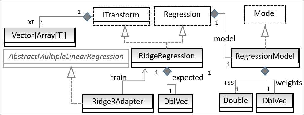
UML class diagram for ridge regression
The UML diagram omits the helper traits or classes such as Monitor or Apache Commons Math components.
Let's look at the training method, train:
def train: RegressionModel = {
  val mlr = new RidgeRAdapter(lambda, xt.head.size) //4

  mlr.createModel(
    xt.map(_.map(implicitly[ToDouble[T]].apply(_))),
    expected
  ) // 5
    RegressionModel(mlr.getWeights, mlr.getRss)  //6
}
It is rather simple; it initialized and executed the regression algorithm implemented in the RidgeRAdapter class (line 4), which acts as an adapter to the internal AbstractMultipleLinearRegression Apache Commons Math library class in the org.apache.commons.math3.stat.regression package (line 5). The method returns a fully initialized regression model, like the ordinary least squared regression (line 6).
Let's look at the adapter class, RidgeRAdapter:
class RidgeRAdapter(
    lambda: Double,
    dim: Int) extends AbstractMultipleLinearRegression {
  var qr: QRDecomposition = _ //7

  def createModel(x: DblMatrix, y: DblVec): Unit ={ //8
    this.newXSampleData(x) //9
    super.newYSampleData(y.toArray)
  }
  def getWeights: Array[Double] = calculateBeta.toArray //10
  def getRss: Double = rss
}
The constructor for the RidgeRAdapter class takes two parameters; the L2 penalty parameter, lambda, and the number of features, dim, in an observation. The QR decomposition in the AbstractMultipleLinearRegression base class does not process the penalty term (line 7). Therefore, the creation of the model has to be redefined in the createModel method (line 8), which needs us to override the newXSampleData method (line 9):
override protected def newXSampleData(x: DblMatrix): Unit =  {
  super.newXSampleData(x)    //11
  val r: RealMatrix = getX
  (0 until dim).foreach(i =>
        r.setEntry(i, i, r.getEntry(i,i) + lambda) ) //12
  qr = new QRDecomposition(r) //13
}
The newXSampleData method overrides the default observations-features matrix r (line 11) by adding the lambda coefficient on its diagonal elements (line 12), then updating the QR decomposition components (line 13).
The weights for the ridge regression model is computed by implemented formula M6 (line 11) in the overridden calculateBeta method (line 10):
override protected def calculateBeta: RealVector =
   qr.getSolver().solve(getY())
The predictive algorithm for the ordinary least squares regression is implemented by the data transformation |>. The method predicts the output value given a model and an input value x (line 14):
def |> : PartialFunction[Array[T], Try[Double]] = {
  case x: Array[T] if(isModel &&
      x.length == model.map(_.size-1).getOrElse(0) =>
        Try(margin(x, model.get) ) //14
}The objective of the test case is to identify the impact of the L2 penalization on the RSS value then compare the predicted values with original values.
Let's consider the first test case related to the regression on the daily price variation of the Copper ETF (symbol: CU) using the stock daily volatility and volume as feature. The implementation of the extraction of observations is identical to that of the least squares regression, described in the previous section:
val LAMBDA: Double = 0.5

for {
  path <- gePath(s"supervised/regression/CU.csv")
  src <- DataSource(path, true, true, 1)  //15
  price <- src.get(adjClose) //16
  volatility <- src.get(volatility) //17
  volume <- src.get(volume) //18
  (features, expected) <- differentialData(
       volatility, volume, price, diffDouble //19
   )
  regression <- RidgeRegression[Double](
       features, expected, LAMBDA //20
  )
} yield {
  if( regression.isModel ) {
    val trend = features.map(
                 margin(_, regression.weights.get) //21
    )
    val y1 = predict(0.2, expected, volatility, volume) //22
    val y2 = predict(5.0, expected, volatility, volume)
    val output = (2 until 10 by 2).map( n =>
          predict(n*0.1, expected, volatility, volume)
    )
  }
}
Let's look at the steps in the execution of the test. It consists of collecting data, extracting the features and expected values, and training the ridge regression model:
- Create a data source extractor for the trading session closing
price, the sessionvolatility, and sessionvolumefor the ETF CU using theDataSourcetransformation (line 15). - Extract the closing
priceof the ETF (line 16), itsvolatilitywithin a trading session (line 17), and tradingvolumeduring the same session (line 18). - Generate the labeled data as a pair of features (relative volatility and relative volume for the ETF) and
expectedoutcome {0, 1} for training the model for which 1 represents price increase and 0 represents price decrease (line 19). The genericdifferentialDatamethod of theXTSeriessingleton is described in the Times series section of Chapter 3, Data Pre-processing. - Instantiate the
RidgeRegressionusing thefeaturesset and theexpectedchange in daily stock price (line 20). - Compute the
trendvalues using themarginfunction of theRegressionModelsingleton (line 21). - Execute a using the ridge regression is implemented by the
predictmethod (line 22):def predict( lambda: Double, deltaPrice: DblVec, volatility: DblVec, volume: DblVec): DblVec = { val observations = zipToSeries(volatility, volume)//25 val regression = new RidgeRegression[Double]( observations, deltaPrice, lambda ) val fnRegr = regression |> //26 observations.map( fnRegr(_).get) //27 }
The observations are extracted from the volatility and volume time series (line 25). The predictive method for the ridge regression, fnRegr (line 26), is applied to each observation (line 27). The RSS value, rss, is plotted for different values of λ, as shown in the following chart:

Graph of RSS versus lambda for copper ETF
The residual sum of squares decreased as λ increases. The curve seems reaching for a minimum around λ=1. The case of λ = 0 corresponds to the least squares regression.
Next, let's plot the RSS value for λ varying between 1 and 100:

Graph RSS versus large value lambda for Copper ETF
This time around, the value of RSS increases with λ, before reaching a maximum for λ > 60. This behavior is consistent with other findings [9:12]. As λ increases, the overfitting gets more expensive and therefore the RSS value increases.
Let's plot the predicted price variation of the copper ETF using ridge regression with a different value of lambda (λ):

Graph of ridge regression on copper ETF price variation with variable lambda
The original price variation of the copper ETF Δ = price(t+1)-price(t) is plotted as lambda =0. Let's analyze the behavior of predictive model for several values of lambda:
- The predicted values for λ = 0.8 are very similar to the original values
- The predicted values for λ = 2 follow the pattern of the original values with reduction of large variations (peaks and troughs).
- The predicted values for λ = 5 correspond to a smoothed dataset. The pattern of the original values is preserved, but the magnitude of the price variation is significantly reduced.
Logistic regression, briefly introduced in the Let's kick the tires section of Chapter 1, Getting Started, is the next logical regression model to discuss. Logistic regression relies on optimization methods. Let's get through a short refresher course in optimization before diving into the logistic regression.