In the Binomial classification section of Chapter 9, Regression and Regularization, you learned the concept of hyperplanes that segregate observations into two classes. These hyperplanes are also known as linear decision boundaries. In the case of the logistic regression, the datasets must be linearly separated. This constraint is particularly an issue for problems with many features that are nonlinearly dependent (high dimension models).
Support vector machines (SVMs) overcome this limitation by estimating the optimal separating hyperplane using kernel functions.
This chapter introduces kernel functions; binary support vectors classifiers, one-class SVMs for anomaly detection, and support vector regression.
In this chapter, you will answer the following questions:
- What is the purpose of kernel functions?
- What is the concept behind the maximization of margin?
- What is the impact of some of the SVM configuration parameters and the kernel method on the accuracy of the classification?
- How do you apply the binary support vector classifier to estimate the risk for a public company to curtail or eliminate its dividend?
- How do you detect outliers with a one-class support vector classifier?
- How does the support vector regression compare to the linear regression?
Every machine learning model introduced in this book so far assumes that observations are represented by a feature vector of a fixed size. However, some real-world applications, such as text mining or genomics, do not lend themselves to this restriction. The critical element of the process of classification is to define a similarity or a distance between two observations. Kernel functions allow developers to compute the similarity between observations without the need to encode them in feature vectors [12:1].
The concept of kernel methods may be a bit odd at first to a novice. Let's consider the simple case of the classification of proteins. Proteins have different lengths and composition, but this does not prevent scientists from classifying them [12:2].
A protein is represented using a traditional molecular notation with which biochemists are familiar. Geneticists describe proteins in terms of a sequence of characters known as the protein sequence annotation. The sequence annotation encodes the structure and composition of the protein. The following picture illustrates the molecular (left) and encoded (right) representation of a protein:

Sequence annotation of a protein
The classification and the clustering of a set of proteins requires the definition of a similarity factor or distance used to evaluate and compare the proteins. For example, the similarity between three proteins can be defined as a normalized dot product of their sequence annotation:

Similarity between the sequence annotations of three proteins
You do not have to represent the entire sequence annotation of the proteins as a feature vector to establish that they belong to the same class. You only need to compare each element of each sequence, one by one, and compute the similarity. For the same reason, the estimation of the similarity does not require the two proteins to have the same length.
In this example, we do not have to assign a numerical value to each element of the annotation. Let's consider an element of the protein annotation as its character c and position p (for example, K, 4). The dot product of the two protein annotations x and x' of the respective lengths n and n' are defined as the number of identical elements (character and position) between the two annotations divided by the maximum length between the two annotations (M1):
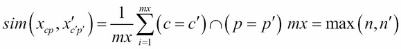
The computation of the similarity for the three proteins produces the result as follows: sim(x,x')=6/12 = 0.50, sim(x,x'')=3/13 =0.23, sim(x',x'')= 4/13= 0.31.
Another similar aspect is that the similarity of two identical annotations is 1.0 and the similarity of two completely different annotations is 0.0.
Note
Visualization of similarity:
It is usually more convenient to use a radial representation to visualize the similarity between features, as in the example of proteins' annotations. The distance d(x,x') = 1/sim(x,x') is visualized as the angle or cosine between two features. The cosine metric is commonly used in text mining.
In this example, the similarity is known as a kernel function in the space of the sequence annotation of proteins.
Although the measure of similarity is very useful when trying to understand the concept of a kernel function, kernels have a broader definition. A kernel K(x, x') is a symmetric, non-negative real function that takes two real arguments (values of two features). There are many different types of kernel functions, among which the most common are:
- The linear kernel (dot product): This is useful in the case of very high-dimensional data, where problems can be expressed as a linear combination of the original features.
- The polynomial kernel: This extends the linear kernel for a combination of features that are not completely linear.
- The radial basis function (RBF): This is the most commonly applied kernel. It is appropriate where the labeled or target data is noisy and requires some level of regularization.
- The sigmoid kernel: This is used in conjunction with neural networks.
- The Laplacian kernel: This is a variant of RBF with a higher regularization impact on training data.
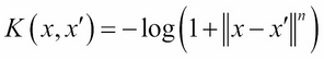
- The log kernel: This is used in image processing.
The simple linear model for regression consists of the dot product of the regression parameters (weights) and the input data (refer to the Ordinary least squares regression section of Chapter 9, Regression and Regularization).
The model is, in fact, the linear combination of weights and linear combination of inputs. The concept can be extended by defining a general regression model as the linear combination of nonlinear functions, known as basis functions (M2):

The most commonly used basis functions are the power and Gaussian functions. The kernel function is described as the dot product of the two vectors of the basis function f(x).f(x') of two features vector x and x'. A partial list of kernel methods is as follows:
M3: The generic kernel function

M4: The linear kernel:

M5: The polynomial kernel with the slope ?, degree n, and constant c:

M6: The sigmoid kernel with the slope ? and constant c:
M7: The radial basis function kernel with the slope ?:
M8: The Laplacian kernel with the slope ?:
M9: The log kernel with the degree n:
The list of discriminative kernel functions described earlier is just a subset of the kernel methods universe. Other types of kernels include:
- Probabilistic kernels: These are kernels derived from generative models. Probabilistic models such as Gaussian processes can be used as a kernel function [12:3].
- Smoothing kernels: This is the nonparametric formulation, averaging density with the nearest neighbor observations [12:4].
- Reproducible kernel Hilbert spaces: This is the dot product of finite or infinite basis functions [12:5].
The kernel functions play a very important role in support vector machines for nonlinear problems.
The concept of kernel function is actually derived from differential geometry and, more specifically, from manifold introduced in the Non-linear models section in Chapter 5, Dimension Reduction.
A manifold is a low dimension features space embedded in the observations space of higher dimension. The dot product (or margin) of two observations, known as the Riemann metric, is computed on a Euclidean tangent space.
The kernel function is the composition of the dot product on the tangent space projected on the manifold using an exponential map, as visualized in the following figure:

Visualization of manifold, Riemann metric, and projection of inner product
A kernel function is the composition g o f of two functions:
- A function h that implements the Riemann metric or similarity between two vectors, v and w
- A function g that implements the projection of the similarity h(v, w) to the manifold (exponential map)
The class KF implements the kernel function as a composition of the function of g and h:
type F1 = Double => Double
type F2 = (Double, Double) => Double

case class KF[G](val g: G, h: F2) {
  def metric(v: DblVec, w: DblVec)
      (implicit gf: G => F1): Double =  //1
    g(v.zip(w).map{ case(_v, _w) => h(_v, _w)}.sum) //2
}
The class KF is parameterized with a type, G, that can be converted to a Function1[Double, Double]. Therefore, the computation of the metric (dot product) requires an implicit conversion from G to Function1 (line 1). The metric is computed by zipping the two vectors, mapping with the h similarity function, and summing the resulting vector (line 2).
Let's define the monadic composition for the class KF:
val kfMonad = new _Monad[KF] {
  override def map[G,H](kf: KF[G])(f: G =>H): KF[H] =
     KF[H](f(kf.g), kf.h) //3
  override def flatMap[G,H](kf: KF[G])(f: G =>KF[H]): KF[H] =
	 KF[H](f(kf.g).g, kf.h)
}
The creation of the instance, kfMonad, overrides the map and flatMap method defined in the generic _Monad trait described in the Abstraction section of Chapter 1, Getting Started. The implementation of the unit method is not essential to the monadic composition and is therefore omitted.
The function argument of the map and flatMap methods applies to the exponential map function g only (line 3). The composition of two kernel functions kf1 = g1 o h and kf2 = g2 o h produces a kernel function kf3 = g2 o (g1 o h) = (g2 o g1) o h = g3 o h.
Note
Interpretation of kernel functions monadic composition:
The visualization of the monadic composition of kernel functions on the manifold is quite intuitive. The composition of two kernel functions consists of composing their respective projection or exponential map functions g. The function g is directly related to the curvature of the manifold around the data point for which the metric is computed. The monadic composition of the kernel functions attempts to adjust the exponential map to fit the curvature of the manifold.
The next step is to define an implicit class to convert a kernel function, of the type KF, to its monadic representation so it can access the map and flatMap methods (line 4):
implicit class kF2Monad[G](kf: KF[G]) {  //4
  def map[H](f: G =>H): KF[H] = kfMonad.map(kf)(f)
  def flatMap[H](f: G =>KF[H]): KF[H] =kfMonad.flatMap(kf)(f)
}
Let's implement the radial basis function, RBF, and the polynomial kernel function, Polynomial, by defining their respective g and h functions. The parameterized type for the kernel function is simply Function1[Double, Double]:
class RBF(s2: Double) extends KF[F1](
    (x: Double) => exp(-0.5*x*x/s2),
    (x: Double, y: Double) => x -y)

class Polynomial(d: Int) extends KF[F1](
    (x: Double) => pow(1.0+x, d),
    (x: Double, y: Double) => x*y)
Here is an example of composition of two kernel functions, a RBF kernel kf1 with standard deviation of 0.6 (line 5) and a polynomial kernel kf2 with a degree 3 (line 6).
val v = Vector[Double](0.5, 0.2, 0.3)
val w = Vector[Double](0.1, 0.7, 0.2)

val composed = for {
  kf1 <- new RBF(0.6)  //5
  kf2 <- new Polynomial(3)  //6
} yield kf2
composed.metric(v, w) //7
Finally, the metric is computed on the composed kernel functions (line 7).