An SVM is a linear discriminative classifier that attempts to maximize the margin between classes during training. This approach is similar to the definition of a hyperplane through the training of the logistic regression (refer to the Binomial classification section of Chapter 9, Regression and Regularization). The main difference is that the support vector machine computes the optimum separating hyperplane between groups or classes of observations. The hyperplane is indeed the equation that represents the model generated through training.
The quality of the SVM depends on the distance, known as margin, between the different classes of observations. The accuracy of the classifier increases as the margin increases.
First, let's apply the support vector machine to extract a linear model (classifier or regression) for a labeled set of observations. There are two scenarios for defining a linear model. The labeled observations are as follows:
- Naturally segregated in the features space (the separable case)
- Intermingled with overlap (the non-separable case)
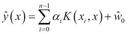
It is easy to understand the concept of an optimal separating hyperplane in case the observations are naturally segregated.
The concept of separating a training set of observations with a hyperplane is better explained with a two-dimensional (x, y) set of observations with two classes, C1 and C2. The label y has the value -1 or +1.
The equation for the separating hyperplane is defined by the linear equation, y=w.xT+w0, which sits in the midpoint between the boundary data points for class C1 (H1 : w.xT + w0 + 1=0) and class C2 (H2 : w.xT + w0 - 1). The planes H1 and H2 are the support vectors:

Visualization of the hard margin in the support vector machine
In the separable case, the support vectors fully segregate the observations into two distinct classes. The margin between the two support vectors is the same for all the observations and is known as the hard margin.
Separable case:
M1: Support vectors equation w is represented as:
M2: Hard margin optimization problem is given by:

In the non-separable case, the support vectors cannot completely segregate observations through training. They merely become linear functions that penalize the few observations or outliers that are located outside (or beyond) their respective support vector, H1 or H2. The penalty variable ?, also known as the slack variable, increases if the outlier is further away from the support vector:

Visualization of the hard margin in the support vector machine
The observations that belong to the appropriate (or own) class do not have to be penalized. The condition is similar to the hard margin, which means that the slack ? is null. This technique penalizes the observations that belong to the class, but are located beyond its support vector; the slack ? increases as the observations get closer to the support vector of the other class and beyond. The margin is then known as a soft margin because the separating hyperplane is enforced through a slack variable.

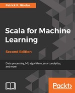
You may wonder how the minimization of the margin error is related to the loss function and the penalization factor introduced for the ridge regression (refer to the Numerical optimization section of Chapter 9, Regression and Regularization). The second factor in the formula corresponds to the ubiquitous loss function. You will certainly recognize the first term as the L2 regularization penalty with ?=1/2C.
The problem can be reformulated as the minimization of a function known as the primal problem [12:6].
M4: Primal problem formulation of the support vector classifier using the L2 regularization:

The C penalty factor is the inverse of the L2 regularization factor. The loss function L is then known as the hinge loss. The formulation of the margin using the C penalty (or cost) parameter is known as the C-SVM formulation. C-SVM is sometimes called the C-Epsilon SVM formulation for the non-separable case.
The ?-SVM (or Nu-SVM) is an alternative formulation to the C-SVM. The formulation is more descriptive than C-SVM; ? represents the upper bound of the training observations that are poorly classified and the lower bound of the observations on the support vectors [12:7].
M5: ?-SVM formulation of a linear SVM using the L2 regularization:
Here, ? is a margin factor used as an optimization variable.
The C-SVM formulation is used throughout the chapters for the binary, one class supports vector classifier as well as the support vector regression.
Note
Sequential Minimal Optimization
The optimization problem consists of the minimization of a quadratic objective function (w2) subject to N linear constraints, N being the number of observations. The time complexity of the algorithm is O(N3 ). A more efficient algorithm, known as Sequential Minimal Optimization (SMO) has been introduced to reduce the time complexity to O(N2 ) (refer to Performance Considerations).
So far, it has been assumed that the separating hyperplane, and therefore the support vectors, are linear functions. Unfortunately, such assumptions are not always correct in the real world.
Support vector machines are known as large or maximum margin classifiers. The objective is to maximize the margin between the support vectors with hard constraints for separable (similarly, soft constraints with slack variables for non-separable) cases.
The model parameters {wi } are rescaled during optimization to guarantee that the margin is at least 1. Such algorithms are known as maximum (or large) margin classifiers.
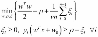
The problem of fitting a nonlinear model into the labeled observations using support vectors is not an easy task. A better alternative consists of mapping the problem to a new, higher dimensional space using a nonlinear transformation. The nonlinear separating hyperplane becomes a linear plane in the new space, as illustrated in the following diagram:
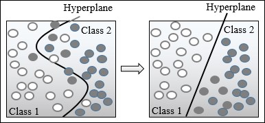
Illustration of the kernel trick in SVM
The nonlinear SVM is implemented using a basis function, f(x). The formulation of the nonlinear C-SVM resembles the formulation of the linear case. The only difference is the constraint along the support vector, using the basis function, f (M6):
The minimization of wT. f(x) in the preceding equation requires the computation of the inner product f(x) T. f(x). The inner product of the basis functions is implemented using one of the kernel functions introduced in the first section. The optimization of the preceding convex problem computes the optimal hyperplane w* as the kernelized linear combination of the training samples, y. f(x), and Lagrange multipliers. This formulation of the optimization problem is known as the SVM dual problem. The description of the dual problem is mentioned as a reference and is well beyond the scope of this book [12:8].
M7: Optimal hyperplane for the SVM dual problem:

M8: Hard margin formulation for the SVM dual problem:

The transformation (x,x') => K(x,x') maps a nonlinear problem into a linear problem in a higher dimensional space. It is known as the kernel trick.
Let's consider, for example, the polynomial kernel defined in the first section with a degree d=2 and coefficient of C0 =1 in a two-dimension space. The polynomial kernel function on two vectors, x=[x1 , x2 ] and z=[x'1 , x'2 ], is decomposed into a linear function in a dimension 6 space:

Tip
Convexity:
Support vector machines can formulate the training of a model as a nonlinear optimization for which the objective function is convex. The drawback is that the kernelization of the SVM may result in many basis functions (higher dimensions). One solution is to reduce the number of basis functions through parameterization, so these functions can adapt to different training sets.
SVMs can be applied to classification, anomaly detection, and regression problems. Let's dive into the support vector classifiers first.
The first classifier to be evaluated is the binary (two-class) support vector classifier. The implementation uses the LIBSVM library created by Chih-Chung Chang and Chih-Jen Lin from the National Taiwan University [12:9].
The library was originally written in C before being ported to Java. It can be downloaded from http://www.csie.ntu.edu.tw/~cjlin/libsvm as a ZIP or tar.gzip file. The library includes the following classifier modes:
- Support vector classifiers (C-SVC, ?-SVC, and one-class SVC)
- Support vector regression (?-SVR and e-SVR)
- RBF, linear, sigmoid, polynomial, and precomputed kernels
LIBSVM has the distinct advantage of using Sequential Minimal Optimization (SMO), which reduces the time complexity of a training of n observations to O(n2 ). LIBSVM documentation covers both the theory and implementation of hard and soft margins and is available at http://www.csie.ntu.edu.tw/~cjlin/papers/guide/guide.pdf.
Note
Why LIBSVM?
There are alternatives to the LIBSVM library for learning and experimenting with SVM. David Soergel from the University of Berkeley refactored and optimized the Java version [12:10]. Thorsten Joachims' SVMLight [12:11] Spark/MLlib includes two Scala implementations of SVM using resilient distributed datasets (refer to Chapter 17, Apache Spark). However, LIBSVM is the most commonly used SVM library.
The implementation of the different support vector classifiers and the support vector regression in LIBSVM is broken down into the following five Java classes:
svm_model: Defines the parameters of the model created during trainingsvm_node: Models the element of the sparse matrix Q, used in the maximization of the marginssvm_parameters: Contains the different models for support vector classifiers and regressions, the five kernels supported in LIBSVM with their parameters, and the weights vectors used in cross-validationsvm_problem: Configures the input to any of the SVM algorithm (number of observations, input vector data x as a matrix, and the vector of labels y)svm: Implements algorithms used in training, classification, and regression
The library also includes template programs for training, prediction, and normalization of datasets.
Tip
The LIBSVM Java code:
The Java version of LIBSVM is a direct port of the original C code. It does not support generic types and is not easily configurable (the code uses switch statements instead of polymorphism). For all its of limitations, LIBSVM is a well-tested and robust Java library for SVM.
Let's create a Scala wrapper to the LIBSVM library to improve its flexibility and ease of use.
The implementation of the support vector machine algorithm uses the design template for classifiers (refer to the Design template for classifier section of the Appendix).
The key components of the implementation of an SVM are as follows:
- A model
SVMModelof the typeModel, which is initialized through training during the instantiation of the classifier. The model class is an adapter to thesvm_modelstructure defined in LIBSVM. - An object
SVMAdapterinterfaces with the internal LIBSVM data structures and methods. - The support vector machine class
SVMis implemented an implicit data transformation of typeITransform.It has three parameters: the configuration wrapper of the typeSVMConfig, the features/time series of the typeXVSeries, and the target or labeled valuesDblVector. - The configuration (the type
SVMConfig) consists of three distinct elements:SVMExecutionthat defines the execution parameters such as maximum number of iterations or convergence criteria,SVMKernelthat specifies the kernel function used during training, andSVMFormulationthat defines the formula (C, epsilon, or nu) used to compute a non-separable case for the support vector classifier and regression.
The key software components of the support vector machine are described in the following UML class diagram:

UML class diagram for the support vector machine
The UML diagram omits the helper traits and classes such as Monitor or Apache commons math components.
LIBSVM exposes several parameters for the configuration and execution of any of the SVM algorithms. Any SVM algorithm is configured with three categories of parameters, which are as follows:
- Formulation (or type) of the SVM algorithms (multiclass classifier, one-class classifier, regression, and so on) using the
SVMFormulationclass - The kernel function used in the algorithm (the RBF kernel, Sigmoid kernel, and so on) using the
SVMKernelclass - Training and execution parameters (convergence criteria, number of folds for cross-validation, and so on) using the
SVMExecutionclass
The instantiation of the configuration consists of initializing the LIBSVM parameter, param, by the SVM type, kernel, and the execution context selected by the user. Each of the SVM parameters case class extends the generic trait, SVMConfigItem:
trait SVMConfigItem { def update(param: svm_parameter): Unit }
The classes inherited from SVMConfigItem are responsible for updating the list of the SVM parameters, svm_parameter, defined in LIBSVM. The update method encapsulates the configuration of the LIBSVM.
The formulation of the SVM algorithm by a class hierarchy with SVMFormulation as base trait:
sealed trait SVMFormulation extends SVMConfigItem {
  def update(param: svm_parameter): Unit
}
The list of formulations for the SVM (C, nu, and eps for regression) is completely defined and known. Therefore, the hierarchy should not be altered and the SVMFormulation trait must be declared sealed. Here is an example of the SVM formulation class, CSVCFormulation, which defines the C-SVM model:
class CSVCFormulation (c: Double) extends SVMFormulation {
   override def update(param: svm_parameter): Unit = {
     param.svm_type = svm_parameter.C_SVC
     param.C = c
  }
}
The other SVM formulation classes, NuSVCFormulation, OneSVCFormulation, and SVRFormulation, implement the ?-SVM, 1-SVM, and e-SVM respectively for regression models.
Next, you need to specify the kernel functions by defining and implementing the SVMKernel trait:
sealed trait SVMKernel extends SVMConfigItem {
  override def update(param: svm_parameter): Unit
}
Once again, there are a limited number of kernel functions supported in LIBSVM. Therefore, the hierarchy of kernel functions is sealed. The following code snippet configures the radius basis function kernel, RbfKernel, as an example of definition of the kernel definition class:
class RbfKernel(gamma: Double) extends SVMKernel {
  override def update(param: svm_parameter): Unit = {
    param.kernel_type = svm_parameter.RBF
    param.gamma = gamma
}
The fact that the LIBSVM Java byte code library is not very extensible does not prevent you from defining a new kernel function in the LIBSVM source code. For example, the Laplacian kernel can be added with the following steps:
- Create a new kernel type in
svm_parameter, such assvm_parameter. LAPLACE = 5. - Add the kernel function name to
kernel_type_tablein thesvmclass. - Add
kernel_type != svm_parameter.LAPLACEto thesvm_check_ parametermethod. - Add the implementation of the kernel function for two values in
svm. kernel_function(Java code):case svm_parameter.LAPLACE: double sum = 0.0; for(int k = 0; k < x[i].length; k++) { final double diff = x[i][k].value - x[j][k].value; sum += diff*diff; } return exp(-gamma*sqrt(sum)); - Add the implementation of the Laplace kernel function in the
svm.k_functionmethod by modifying the existing implementation of RBF (distanceSqr). - Rebuild the
libsvm.jarfile.
The SVMExecution class defines the configuration parameters for the execution of the training of the model, namely, the convergence factor, eps for the optimizer (line 2), the size of the cache cacheSize (line 1), and the number of folds, nFolds used during cross-validation:
class SVMExecution(cacheSize: Int, eps: Double, nFolds: Int)
extends SVMConfigItem {
  override def update(param: svm_parameter): Unit = {
    param.cache_size = cacheSize //1
    param.eps = eps //2
  }
}
Cross-validation is performed only if the nFolds value is greater than 1. We are finally ready to create the configuration class, SVMConfig, which hides and manages all of the different configuration parameters:
class SVMConfig(formula: SVMFormulation, kernel: SVMKernel,
     exec: SVMExecution) {
  val param = new svm_parameter
  formula.update(param) //3
  kernel.update(param)  //4
  exec.update(param)  //5
}
The class SVMConfig delegates the selection of the formula to the SVMFormulation class (line 3), selection of the kernel function to SVMKernel class (line 4), and the execution parameters to SVMExecution class (line 5). The sequence of update calls initializes the LIBSVM list of configuration parameters.
We need to create an adapter object to encapsulate the invocation to LIBSVM. The object SVMAdapter hides the LIBSVM internal data structures, svm_model and svm_node:
object SVMAdapter {
  type SVMNodes = Array[Array[svm_node]]
  class SVMProblem(numObs: Int, expected: Array[Double]) //6

  def createSVMNode(dim: Int,
                 x: Array[Double]): Array[svm_node] //7
  def predictSVM(model: SVMModel, x: Array[Double]): Double//8
  def crossValidateSVM(
     problem: SVMProblem, //9
     param: svm_parameter,
     nFolds: Int,
     expected: Array[Double])
  def trainSVM(
     problem: SVMProblem,  //10
     param: svm_parameter): svm_model
}
The object SVMAdapter is a single-entry point to LIBSVM for training, validating an SVM model, and executing predictions:
SVMProblemwraps the definition of the training objective or problem in LIBSVM, using the labels orexpectedvalues (line 6)createSVMNodecreates a new computation node for each observationx(line 7)predictSVMpredicts the outcome of a new observationxgiven a model,svm_modelgenerated through training (line 8)crossValidateSVMvalidates the model,svm_modelwith anFoldtraining – validation sets (line 9)trainSVMexecutes the training configuration, problem (line 10).
The model for SVM is defined with the following two components:
svm_modelthat is the SVM model parameters defined in LIBSVMaccuracythat is the accuracy of the model computed during cross-validation:case class SVMModel(svmmodel: svm_model, accuracy: Double) extends Model { lazy val residuals: Array[Double] = svmmodel.sv_coef(0) }
The residuals r = y – f(x) are computed in the LIBSVM library.
Tip
Accuracy in SVM model:
You may wonder why the value of the accuracy is a component of the model. The accuracy component of the model provides the client code with a quality metric associated with the model. Integrating the accuracy into the model allows the user to make informed decision in accepting or rejecting the model. The accuracy is stored in the model file for subsequent analysis.
Next, let's create the first support vector classifier for the two-class problems. The SVM class implements the monadic data transformation ITransform that generates implicitly a model from a training set as described in the Monadic data transformation
section in Chapter 2, Data Pipelines
(line 11).
The constructor for SVM follows the template described in the Design template for classifiers section of Appendix. It takes a configuration of type SVMConfig, a set of observations xt of type Array[T], and a set of labels (expected values) of type, DblVec as arguments (line 12):
class SVM[T: ToDouble](
  config: SVMConfig,
  xt: Vector[Array[T]],
  expected: DblVec)  //12
extends ITransform[Array[T],Double]{ //11

  val normEPS = config.eps*1e-7 //13
  val model: Option[SVMModel] = train //14

  def accuracy: Option[Double] = model.map( _.accuracy) //15
  def mse: Option[Double] //16
  def margin: Option[Double] //17
}
The normEPS is used for rounding errors in the computation of the margin (line 13). The model of type SVMModel is generated through training by the SVM constructor (line 14). The last four methods are used to compute the parameters of the model accuracy (line 15), the mean square of errors, mse (line 16), and the margin (line 17).
Let's look at the training method, train:
def train: Option[SVMModel] = Try {
  val problem = new SVMProblem(xt.size, expected.toArray) //18
  val dim = dimension(xt)
  xt.indices.foreach(
    n => problem.update(n, createNode(dim,x(n)).map((c(_)))))//12
  )
  new SVMModel(
     trainSVM(problem, config.param),accuracy(problem) //20
  )
}.toOption
The train method creates a SVMProblem that provides LIBSVM with training components (line 18). The purpose of the SVMProblem class is to manage the definition of training parameters implemented in LIBSVM, as follows:
class SVMProblem(numObs: Int, expected: Array[Double]) {
  val problem = new svm_problem //21
  problem.l = numObs
  problem.y = expected
  problem.x = new SVMNodes(numObs)

  def update(n: Int, node: Array[svm_node]): Unit =
     problem.x(n) = node //22
}
The arguments of the SVMProblem constructor, the number of observations and the labels or expected values are used to initialize the corresponding data structure, svm_problem in LIBSVM (line 21). The method update maps each observation, defined as an array of svm_node to the problem (line 22).
The method createNode creates an array of svm_node from an observation. A svm_node in LIBSVM is the pair of the index j of a feature in an observation (line 23) and its value y (line 24):
def createNode(dim: Int,x: Array[Double]): Array[svm_node] =
   x.indices./:(new Array[svm_node](dim)){(newNode, j) =>
     val node = new svm_node
     node.index= j	//23
     node.value = x(j)	//24
     newNode(j) = node
     newNode
   }
The mapping between an observation and a LIBSVM node is illustrated in the following diagram:

Indexing of observations using LIBSVM
The method trainSVM pushes the training request with a well-defined problem and configuration parameters to LIBSVM by invoking the svm_train method (line 26):
def trainSVM(problem: SVMProblem,
            param: svm_parameter): svm_model =
 svm.svm_train(problem.problem, param) //26
The accuracy is the ratio of true positive plus the true negative over the size of the test sample (refer to the Key metrics section of Chapter 2, Data Pipelines). It is computed through cross-validation only if the number of folds is initialized in the SVMExecution configuration class as greater than 1. Practically, the accuracy is computed by invoking the cross-validation method, svm_cross_validation, in the LIBSVM package, and then computing the ratio of the number of predicted values that match the labels over the total number of observations:
def accuracy(problem: SVMProblem): Double =
  if( config.isCrossValidation ) {
     val target = crossValidateSVM(problem, config.param,  //27
                             config.nFolds, expected.size)

     target.view.zip(expected.view)
             .count{ case(x, y) => abs(x-y) < config.eps }//28
             .toDouble/expected.size
  }
  else 0.0
The call to the crossValidateSVM method of SVMAdapter forwards the configuration and execution of the cross validation with config.nFolds (line 27):
def crossValidateSVM(
  problem: SVMProblem,
  param: svm_parameter,
  nFolds: Int,
  size: Int) = {
    val target = Array.fill(size)(0.0)
    svm.svm_cross_validation(
       problem.problem, param, nFolds, target)
    )
    target
}
The Scala filter weeds out the observations that were poorly predicted (line 28). This minimalist implementation is good enough to start exploring the support vector classifier.
The implementation of the classification method |> for the SVM class follows the same pattern as the other classifiers. It invokes the predictSVM method in SVMAdapter that forwards the request to LIBSVM (line 29):
override def |> : PartialFunction[Array[T], Try[Double]] =  {
   case x: Array[T] if(x.size == dimension(xt) && isModel) =>
     Try(predictSVM(model.get, x.map(c(_))) )  //29
}
The first evaluation consists of understanding the impact of the penalty factor C to the margin in the generation of the classes. Let's implement the computation of the margin. The margin is defined as 2/|w| and implemented as a method of the SVM class, as follows:
def margin: Option[Double] = model.map{ m =>
   1.0/sqrt(m.residuals.reduce(_ * _))
}
The first instruction computes the sum of the squares, wNorm, of the residuals r = y – f(x|w). The margin is ultimately computed if the sum of squares is significant enough to avoid rounding errors.
The margin is evaluated using an artificially generated time series and labeled data. First, we define the method to evaluate the margin for a specific value of the penalty (inversed regularization coefficient) factor C:
val GAMMA = 0.8; val CACHE_SIZE = 1<<8
val NFOLDS = 2; val EPS = 1e-5

def evalMargin(features: Vector[Array[Double]],
               expected: DblVec,
               c: Double): Int = {
  val execEnv = SVMExecution(CACHE_SIZE, EPS, NFOLDS)
  val config = SVMConfig(new CSVCFormulation(c),
                        new RbfKernel(GAMMA),
                        execEnv
               )
  val svc = SVM[Double](config, features, expected)
  svc.margin.map(_.toString) //30
}
The method evalMargin uses the execution parameters, CACHE_SIZE, EPS, and NFOLDS. The execution displays the value of the margin for different values of C (line 30). The method is invoked iteratively to evaluate the impact of the penalty factor on the margin extracted from the training of the model. The test uses a synthetic time series to highlight the relation between C and the margin. The synthetic time series created by the method generate consists of two training sets of an equal size, N:
- Data points generated as y = x(1 + r/5) for the label 1, r being a randomly generated number over the range [0,1] (line 31)
- Randomly generated data point y = r for the label of -1 (line 32)
def generate: Option[(Vector[Array[Double]],Array[Double])] = {
  val z = Vector.tabulate(N)(i => {
     val ri = i*(1.0 + 0.2*nextDouble)
     Array[Double](i, ri)  //31
  }) ++
  Vector.tabulate(N)(i =>Array[Double](i,i*nextDouble))

  normalizeArray(z).map(
     (_, Array.fill(N)(1) ++ Array.fill(N)(-1))
  ).toOption  //32
}
The evalMargin method is executed for values C ranging from 0.1 to 5:
generate.map(y =>
  (0.1 until 5.0 by 0.1)
    .flatMap(evalMargin(y._1, y._2, _)).mkString("
")
)
Tip
val versus final val:
There is a difference between a val and a final val. A non-final value can be overridden in a subclass. Overriding a final value produces a compiler error, as follows:
class A { val x = 5;  final val y = 8 }
class B extends A {
  override val x = 9 // OK
  override val y = 10 // Error
}
The following chart illustrates the relation between the penalty, or cost factor, C, and the margin:

The margin value versus C-penalty factor for a support vector classifier
As expected, the value of the margin decreases as the penalty term C increases. The C penalty factor is related to the L2 regularization factor ? as C ~ 1/?. A model with a large value of C has a high variance and a low bias, while a small value of C will produce lower variance and a higher bias.
The next test consists of comparing the impact of the kernel function on the accuracy of the prediction. Once again, a synthetic time series is generated to highlight the contribution of each kernel. The test code uses the runtime prediction or classification method |> to evaluate the different kernel functions. Let's create a method to evaluate and compare these kernel functions. All we need is the following (line 33):
- A training set,
xt, of typeVector[Array[Double]] - A test set,
test, of typeVector[Array[Double]] - A set of
labelsfor the training set, taking the value 0 or 1 - A kernel function
kF
Consider the following code:
val C = 1.0
def accuracy(
  xt: Vector[Array[Double]],
  test: Vector[Array[Double]],
  labels: DblVec,
  kF: SVMKernel): Double = { //33

  val config = SVMConfig(new CSVCFormulation(C), kF) //34
  val svc = SVM[Double](config, xt, labels)
  val pfnSvc = svc |> //35

  test.zip(labels).count{ case(x, y) =>
    if(pfnSvc.isDefinedAt(x)) pfnSvc(x).get == y else false
  }.toDouble/test.size //36
}
The configuration, config, of the SVM uses C penalty factor 1, the C-formulation, and the default execution environment (line 34). The predictive partial function pfnSvc (line 35) is used to compute the predictive values for the test set. Finally, the method accuracy counts the number of successes for which the predictive values match the labeled or expected values. The accuracy is computed as the ratio of the successful prediction over the size of the test sample (line 36).
In order to compare the different kernels, let's generate three datasets of the size 2N for a binomial classification using the pseudo-random data generation method genData:
def genData(
  variance: Double,
  mean: Double): Vector[Array[Double]] = {

  val rGen = new Random(System.currentTimeMillis)
  Vector.tabulate(N){ _ =>
    rGen.setSeed(rGen.nextLong)
    Array[Double](rGen.nextDouble, rGen.nextDouble)
        .map(variance*_ - mean)  //37
  }
}
The random value is computed through a transformation f(x) = variance*x = mean (line 37). The training and test sets consist of the aggregation of two classes of data points:
- Random data points with
varianceaandmeanbassociated to the label 0.0 - Random data points with
variance aandmean 1-bassociated to the label 1.0
Consider the following code for the training set:
val trainSet = genData(a, b) ++ genData(a, 1-b)
val testSet = genData(a, b) ++ genData(a, 1-b)
The parameters a, b are selected from two groups of training data points with various degree of separation to illustrate the separating hyperplane.
The following chart describes the high margin; the first training set generated with the parameters a = 0.6 and b = 0.3 illustrates the highly separable classes with a clean and distinct hyperplane:

Scatter plot for training and testing sets with a = 0.6 and b = 0.3
The following chart describes the medium margin; the parameters a = 0.8 and b = 0.3 generate two groups of observations with some overlap:

Scatter plot for training and testing sets with a = 0.8 and b = 0.3
The following chart describes the low margin; the two groups of observations in this last training are generated with a = 1.4 and b = 0.3 and show a significant overlap:

Scatter plot for training and testing sets with a = 1.4 and b = 0.3
The test set is generated in a similar fashion as the training set, as they are extracted from the same data source:
val GAMMA = 0.8; val COEF0 = 0.5; val DEGREE = 2 //38
val N = 100

def compareKernel(a: Double, b: Double) {
  val labels = Vector.fill(N)(0.0) ++ Vector.fill(N)(1.0)

  evalKernel(trainSet, testSet,labels,new RbfKernel(GAMMA))
  evalKernel(trainSet, testSet, labels,
      new SigmoidKernel(GAMMA))
  evalKernel(trainSet, testSet, labels, LinearKernel)
  evalKernel(trainSet, testSet, labels,
      new PolynomialKernel(GAMMA, COEF0, DEGREE))
}
The parameters for each of the four kernel functions are arbitrary selected from textbooks (line 38). The evalKernel method defined earlier is applied to the three training sets: high margin (a = 1.4), medium margin (a = 0.8), and low margin (a = 0.6), with each of the four kernels (RBF, sigmoid, linear, and polynomial). The accuracy is assessed by counting the number of observations correctly classified for all the classes for each invocation of the predictor, |>:

Comparative chart of kernel functions using synthetic data
Although the different kernel functions do not differ in terms of their impact on the accuracy of the classifier, you can observe that the RBF and polynomial kernels produce results that are slightly more accurate. As expected, the accuracy decreases as the margin decreases. A decreasing margin is a sign that the cases are not easily separable, affecting the accuracy of the classifier:

Impact of the margin value on the accuracy of RBF and Sigmoid kernel functions
In summary, there are four steps in creating an SVC-based model:
- Select a features-set.
- Select the C-penalty (inverse regularization).
- Select the kernel function.
- Tune the kernel parameters
Note
Test case design:
The test to compare the different kernel methods is highly dependent on the distribution or mixture of data in the training and test sets. The synthetic generation of data in this test case is used for illustrating the margin between classes of observations. Real-world datasets may produce different results.
As mentioned earlier, this test case relies on synthetic data to illustrate the concept of margin and compare kernel methods. Let's use the support vector classifier for a real-world financial application.
The purpose of the test case is to evaluate the risk for a company to curtail or eliminate its quarterly or yearly dividend. The features selected are financial metrics relevant to a company's ability to generate cash flow and pay out its dividends over the long term.
We need to select any subset of the following financial technical analysis metrics (refer to the Metrics section of the Appendix):
- Relative change in stock prices over the last 12 months
- Long-term debt-equity ratio
- Dividend coverage ratio
- Annual dividend yield
- Operating profit margin
- Short interest (ratio of shares shorted over the float)
- Cash per share-share price ratio
- Earnings per share trend
The earnings trend has the following values:
- -2, if earnings per share decline by more than 15 percent over the last 12 months
- -1, if earnings per share decline between 5 percent and 15 percent
- 0, if earning per share is maintained within 5 percent
- +1, if earnings per share increase between 5 percent and 15 percent
- +2, if earnings per share increase by more than 15 percent, the values are normalized with values 0 and 1
The labels or expected output, dividend changes, is categorized as follows:
- -1, if dividend is cut by more than 5 percent
- 0, if dividend is maintained within 5 percent
- +1, if dividend is increased by more than 5 percent
Let's combine two of these three labels, {-1, 0, 1}, to generate two classes for the binary SVC:
- Class C1 = stable or decreasing dividends and class C2 = increasing dividends; represented by
dividendsA - Class C1 = decreasing dividends and class C2 = stable or increasing dividends; represented by
dividendsB
The different tests are performed with a fixed set of configuration parameters C and GAMMA and a two-fold validation configuration:
val path = "supervised/svm/dividends2.csv"
val C = 1.0
val GAMMA = 0.5
val EPS = 1e-2
val NFOLDS = 2

val extractor = relPriceChange :: debtToEquity ::
    dividendCoverage :: cashPerShareToPrice :: epsTrend ::
    shortInterest :: dividendTrend ::
    List[Array[String] =>Double]()  //39

val pfnSrc = DataSource(path, true, false,1) |> //40
val config = SVMConfig(new CSVCFormulation(C),
     new RbfKernel(GAMMA), SVMExecution(EPS, NFOLDS))

for {
  path <- getPath(dataPath)
  pfnSrc <- DataSource(path, true, false, 1) //40
  input <- pfnSrc.|>(extractor) //41
  obs <- getObservations(input) //42
} yield {
  svc = SVM[Double](config, obs, input.last.toVector)
  show(s"${svc.toString}
accuracy=${svc.accuracy.getOrElse(-1)}")
}
The first step is to define the extractor, that, is the list of fields to retrieve from the file, dividends2.csv (line 39). The partial function pfnSrc generated by the DataSource transformation class (line 40) converts the input file into a set of typed fields (line 41). An observation is an array of fields. The sequence of observations, obs, are generated from the input fields by transposing the matrix observations x features (line 42):
def getObservations(input: Vector[Array[Double]]):
     Try[Vector[Array[Double]]] = Try {
  transpose( input.dropRight(1).map(_.toArray) ).toVector
}
The test computes the model parameters and the accuracy from the cross-validation during the instantiation of SVM.
Tip
LIBSVM scaling:
LIBSVM supports feature normalization known as scaling, prior to training. The main advantage of scaling is to avoid attributes in greater numeric ranges dominating those in smaller numeric ranges. Another advantage is to avoid numerical difficulties during the calculation. In our examples, we use the normalization method of the time series normalize. Therefore, the scaling flag in LIBSVM is disabled.
The test is repeated with a different set of features and consists of comparing the accuracy of the support vector classifier for different features sets. The features sets are selected from the content of the .csv file by assembling the extractor with different configurations, as follows:
val extractor = … :: dividendTrend :: ....
The following bar chart displays the various values of the accuracy of the different SVM models, using the training set A.

Comparative study of trading strategies using binary SVC
The test demonstrates that the selection of the proper features set is the most critical step in applying the SVM, or any other model for that matter, to classification problems. In this case, the accuracy is also affected by the small size of the training set. The increase in the number of features also reduces the contribution of each specific feature to the loss function.
The same process is repeated for the test B whose purpose is to classify companies with decreasing dividends and companies with stable or increasing dividends, as shown in the following graph:

Comparative study of trading strategies using binary SVC
The difference, in terms of accuracy of prediction, between the first three features set and the last two features set in the preceding graph is more pronounced in test A than in test B. In both tests, the feature eps (earning per share) trend improves the accuracy of the classification. It is a particularly good predictor for companies with increasing dividends.
The problem of predicting the distribution (or not) dividends can be restated as evaluating the risk of a company to dramatically reduce its dividends.
What is the risk a company eliminates its dividend altogether? Such a scenario is rare, and those cases are outliers. A one-class support vector classifier can be used to detect outliers or anomalies [12:13].
The design of the one-class SVC is an extension of the binary SVC. The main difference is that a single class contains most of the baseline (or normal) observations. A reference point, known as the SVC origin, replaces the second class. The outliers (or abnormal) observations reside beyond (or outside) the support vector of the single class:

Visualization of the one-class SVC
The outlier observations have a labeled value of -1, while the remaining training sets are labeled +1. To create a relevant test, we add four more companies that have drastically cut their dividends (ticker symbols WLT, RGS, MDC, NOK, and GM). The dataset includes the stock prices and financial metrics recorded prior to the cut in dividends.
The implementation of this test case is very similar to the binary SVC driver code, except for the following:
The test is executed against the dataset resources/data/svm/dividends2.csv. First, we need to define the formulation for the one-class SVM:
class OneSVCFormulation(nu: Double) extends SVMFormulation {
  override def update(param: svm_parameter): Unit = {
    param.svm_type = svm_parameter.ONE_CLASS
    param.nu = nu
  }
}
The test code is similar to the execution code for the binomial SVC. The only difference is the definition of the output labels; -1 for companies eliminating dividends and +1 for all other companies:?
val NU = 0.2
val GAMMA = 0.5
val EPS = 1e-3
val NFOLDS = 2

val extractor = relPriceChange :: debtToEquity ::
   dividendCoverage :: cashPerShareToPrice :: epsTrend ::
   dividendTrend :: List[Array[String] =>Double]()

val filter = (x: Double) => if(x == 0) -1.0 else 1.0  //43
val pfnSrc = DataSource(path, true, false, 1) |>
val config = SVMConfig(new OneSVCFormulation(NU),  //44
    new RbfKernel(GAMMA), SVMExecution(EPS, NFOLDS))
for {
  pfn <- pfnSrc
  input <- pfn(extractor)
  obs <- getObservations(input)
} yield {
  svc = SVM[Double](
    config, obs, input.last.map(filter(_)).toVector
  )
}
The labels or expected data are generated by applying a binary filter to the last field, dividendTrend (line 43). The formulation in the configuration has the type OneSVCFormulation (line 44).
The model is generated with an accuracy of 0.821. This level of accuracy should not be a surprise; the outliers (companies that eliminated their dividends) are added to the original dividend .csv file. These outliers differ significantly from the baseline observations (companies who have reduced, maintained, or increased their dividend) in the original input file.
Where the labeled observations are available, the one-class SVM is an excellent alternative to clustering techniques.
Note
Definition of anomaly:
The results generated by a one-class support vector classifier depend heavily on the subjective definition of an outlier. The test case assumes that the companies that eliminate their dividends have unique characteristics that set them apart, and are different even from companies who have cut, maintained, or increased their dividend. There is no guarantee that this assumption is indeed always valid.
Most of the applications using support vector machines are related to classification. However, the same technique can be applied to regression problems. Luckily, as with classification, LIBSVM supports two formulations for support vector regression:
- e-SVR (sometimes called C-SVR)
- ?-SVR
For the sake of consistency with the two previous cases, the following test uses the ? (or C) formulation of the support vector regression.
The SVR introduces the concept of error insensitive zone and insensitive error, e. The insensitive zone defines a range of values around the predictive values, y(x). The penalization component C does not affect the data point {xi ,yi } that belongs to the insensitive zone [12:14].
The following diagram illustrates the concept of an error insensitive zone, using a single variable feature x and an output y. In the case of a single variable feature, the error insensitive zone is a band of width 2e (e is known as the insensitive error). The insensitive error plays a similar role to the margin in the SVC:

Visualization of the support vector regression and insensitive error
For the mathematically inclined, the maximization of the margin for nonlinear models introduces a pair of slack variables. As you may remember, the C-support vector classifiers use a single slack variable. The preceding diagram illustrates the minimization formula.
M9: e-SVR formulation:

Here, e is the insensitive error function.
M10: The e-SVR regression equation:
Let's reuse the SVM class to evaluate the capability of the SVR, compared to the linear regression (refer to the Ordinary least squares regression section of Chapter 9, Regression and Regularization).
This test consists of reusing the example that illustrates the presented in single-variate linear regression (refer to the One-variate linear regression section of Chapter 9, Regression and Regularization). The purpose is to compare the output of the linear regression with the output of the SVR for predicting the value of a stock price or an index. We select the S&P 500 exchange traded fund, SPY, which is a proxy for the S&P 500 index.
The model consists of the following:
- One labeled output: SPY-adjusted daily closing price
- One single variable feature set: the index of the trading session (or index of the values SPY)
The implementation follows a familiar pattern:
- Define the configuration parameters for the SVR (the C cost/penalty function,
GAMMAcoefficient for the RBF kernel, EPS for the convergence criteria, andEPSILONfor the regression insensitive error) - Extract the labeled data (SPY
price) from the data source (DataSource), which is the Yahoo financials CSV-formatted data file - Create the linear Regression,
SingleLinearRegression, with the index of the trading session as the single variable feature and the SPY-adjusted closing price as the labeled output - Create the observations as a time series of indexes,
xt - Instantiate the SVR with the index of trading session as features and the SPY adjusted closing price as the labeled output
- Run the prediction methods for both SVR and the linear regression and compare the results of the linear regression and SVR,
collect:val C = 12 val GAMMA = 0.3 val EPSILON = 2.5 val config = SVMConfig( new SVRFormulation(C, EPSILON), new RbfKernel(GAMMA) //45 ) for { src <- DataSource(path, false, true, 1) price <- src.get(close) (xt, y) <- getLabeledData(price.size) //46 linRg <- SingleLinearRegression[Double](price, y) //47 } yield { val svr = SVM[Double](config, xt, price) collect(svr, linRg, price) }
The formulation in the configuration has the type SVRFormulation (line 45). The DataSource class extracts the price of the SPY ETF. The method getLabeledData generates the input features xt and the labels (or expected values) y (line 46):
type LabeledData = (Vector[Array[Double]], DblVec)

def getLabeledData(numObs: Int): Try[LabeledData ] = Try {
  val y = Vector.tabulate(numObs)(_.toDouble)
  val xt = Vector.tabulate(numObs)(Array[Double](_))
  (xt, y)
}
The single variate linear regression, SingleLinearRegression, is instantiated using the input price and labels y as input (line 47).
Finally, the method collect executes the two regression partial functions; pfSvr and pfLinr:
def collect(
   svr: SVM[Double],
   linr: SingleLinearRegression[Double],
   price: DblVec): List[Vector[DblPair]] = {

  val pfSvr = svr |>
  val pfLinr = linr |>
  (0 until price.size-80).foreach( n =>
    for {
  	   val z = Array[Double](n.toDouble)
      if( pfSvr.isDefinedAt(z)); x <- pfSvr(z)
      if( pfLin.isDefinedAt(n)); y <- pfLinr(n)
  	 } yield  {  ... }
  })
  ….
}
The results are displayed in the following graph, generated using the JFreeChart library. The code to plot the data is omitted because it is not essential to the understanding of the application:

Comparative plot of linear regression and SVR
The support vector regression provides a more accurate prediction than the linear regression model. You can also observe that the L2 regularization term of the SVR penalizes the data points (the SPY price) with a high deviation from the mean of the price. A lower value of C will increase the L2-norm penalty factor as ? =1/C.
There is no need to compare SVR with logistic regression, as logistic regression is a classifier. However, SVM is related to logistic regression; the hinge loss in SVM is similar to the loss in the logistic regression [12:15].