Genetic algorithms have the following three components:
- Genetic encoding (and decoding): This is the conversion of a solution candidate and its components into binary format (an array of bits or a string of 0 and 1 characters)
- Genetic operations: This is the application of a set of operators to extract the best (most genetically fit) candidates (chromosomes)
- Genetic fitness function: This is the evaluation of the fittest candidate using an objective function
Encodings and the fitness function are problem-dependent. Genetic operators are not.
Let's consider the optimization problem in machine learning that consists of maximizing the log likelihood or minimizing the loss function. The goal is to compute the parameters or weights, w={wi}, that minimize or maximize a function f(w). In the case of a nonlinear model, variables may depend on other variables, which make the optimization problem particularly challenging.
The genetic algorithm manipulates variables as bits or bit strings. The conversion of a variable into a bit string is known as encoding. In cases where the variable is continuous, the conversion is known as quantization or discretization. Each type of variable has a unique encoding scheme, as follows:
- Boolean values are easily encoded with 1 bit: 0 for false and 1 for true.
- Continuous variables are quantized or discretized like the conversion of an analog to a digital signal. Let's consider the function with a maximum max (similarly min for minimum) over a range of values, encoded with n=16 bits:

Illustration of quantization of continuous variable y = f(x)
The step size of the discretization is computed as (M1):
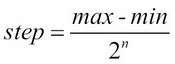
The step size of the quantization of the sine y = sin(x) in 16-bits is 1.524e-5.
Discrete or categorical variables are a bit more challenging to encode to bits. At a minimum, all the discrete values must be accounted for. However, there is no guarantee that the number of variables will coincide with the bit boundary:

Padding for base 2 representation of values
In this case, the next exponent, n+1, defines the minimum number of bits required to represent the set of values: n = log2(m).toInt + 1. A discrete variable with 19 values requires five bits. The remaining bits are set to an arbitrary value (0, NaN…) depending on the problem. This procedure is known as padding.
Encoding is as much an art as it is a science. For each encoding function, you need a decoding function to convert the binary representation back to actual values.
A predicate for a variable x is a relation defined as 'x operator [target]', for instance, 'unit cost < [$9]', 'temperature = [82F]', or 'movie rating is [3 stars]'.
The simplest encoding scheme for predicates is as follows:
- Variables are encoded as a category or type (for example, temperature, barometric pressure, and so on) because there is a finite number of variables in any model
- Operators are encoded as discrete type
- Values are encoded as either discrete or continuous values
Note
Encoding format for predicates:
There are many approaches for encoding a predicate in a binary string. For instance, the format {operator, left-operand, right-operand} is useful because it allows you to encode a binary tree. The entire rule, IF predicate THEN action, can be encoded with the action being represented as a discrete or categorical value.
The solution encoding approach describes the solution to a problem as an unordered sequence of predicates. Let's consider the following rule:
IF {Gold price rises to [1316$/ounce]} AND
   {US$/Yen rate is [104]}).
THEN {S&P 500 index is [UP]}
In this example, the search space is defined by two levels:
- Boolean operators (for example, AND) and predicates
- Each predicate is defined as a tuple {variable, operator, target value}
The tree representation for the search space is shown in the following diagram:

Graph representation of encoded rules
The binary string representation is decoded back to its original format for further computation:
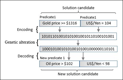
Encoding, alteration, and decoding predicates
There are two approaches to encoding such a candidate solution or a chain of predicates:
- Flat encoding of a chromosome
- Hierarchical coding of a chromosome as a composition of genes
The flat encoding approach consists of encoding the set of predicates into a single chromosome (bits string) representing a specific solution candidate to the optimization problem. The identity of the predicates is not preserved:

Flat addressing schema for chromosomes
A genetic operator manipulates the bits of the chromosome regardless of whether the bits refer to a specific predicate:

Chromosome encoding with flat addressing
In this configuration, the characteristic of each predicate is preserved during the encoding process. Each predicate is converted into a gene represented by a bit string. The genes are aggregated to form the chromosome. An extra field is added to the bit string or chromosome for the selection of the gene. This extra field consists of the index or the address of the gene:

Hierarchical addressing schema for chromosomes
A generic operator selects the predicate it needs to manipulate first. Once the target gene is selected, the operator updates the binary string associated to the gene, as follows:

Chromosome encoding with flat addressing
The next step is to define the genetic operators that manipulate or update the binary string representing either a chromosome or individual genes.
The implementation of the reproduction cycle attempts to replicate the natural reproduction process [10:7]. The reproduction cycle that controls the population of chromosomes consists of three genetic operators:
- Selection: This operator ranks chromosomes according to a fitness function or criteria. It eliminates the weakest or less-fit chromosomes and controls the population growth.
- Crossover: This operator pairs chromosomes to generate offspring chromosomes. These offspring chromosomes are added to the population along with their parent chromosomes.
- Mutation: This operator introduces a minor alteration in the genetic code (binary string representation) to prevent the successive reproduction cycles from electing the same fittest chromosome. In optimization terms, this operator reduces the risk of the genetic algorithm converging quickly towards a local maximum or minimum.
Tip
Transposition operator:
Some implementations of genetic algorithms use a fourth operator, genetic transposition, in cases where the fitness function cannot be very well defined and the initial population is very large. Although additional genetic operators could potentially reduce the odds of finding a local maximum or minimum, the inability to describe the fitness criteria or the search space is a sure sign that a genetic algorithm may not be the most suitable tool.
The following diagram gives an overview of the genetic algorithm workflow:

Basic workflow for the execution of genetic algorithms
The reproduction cycle can be implemented as a recursion or iteratively. The encoding and decoding operations are defined as a pair of transform and inverse transform from a Scala object to a bit string and vice-versa.
Tip
Initialization
The initialization of the search space (a set of potential solutions to a problem) in any optimization procedure is challenging, and genetic algorithms are no exception. In the absence of bias or heuristics, the reproduction initializes the population with randomly generated chromosomes. However, it is worth the effort to extract the characteristics of a population. Any well-founded bias introduced during initialization facilitates the convergence of the reproduction process.
Each of these genetic operators has at least one configurable parameter that has to be estimated and/or tuned. Moreover, you will likely need to experiment with different fitness functions and encoding schemes to increase your odds of finding a fittest solution (or chromosome).
The purpose of the genetic selection phase is to evaluate, rank, and weed out the chromosomes (that is, the solution candidates) that are not a good fit for the problem. The selection procedure relies on a fitness function to score and rank candidate solutions through their chromosomal representation. It is a common practice to constrain the growth of the population of chromosomes by setting a limit to the size of the population.
There are several methodologies to implement the selection process, from scaled relative fitness, Holland roulette wheel, and tournament selection to rank-based selection [10:8].
Note
Relative fitness degradation
As the initial population of chromosomes evolves, the chromosomes tend to get more and more similar to each other. This phenomenon is a healthy sign that the population is converging. However, for some problems, you may need to scale or magnify the relative fitness to preserve a meaningful difference in the fitness score between the chromosomes [10:9].
The following implementation relies on rank-based selection. The selection process consists of the following steps:
- Apply the fitness function to each chromosome j in the population, fj.
- Compute the total fitness score for the entire population, ?fj.
- Normalize the fitness score of each chromosome by the sum of the fitness scores of all the chromosomes, fj = fi/Sfj.
- Sort the chromosomes by their descending fitness score, fj < fj-1.
- Compute the cumulative fitness score for each chromosome, j fj = fj + ?fk.
- Generate the selection probability (for the rank-based formula) as a random value, p e [0,1].
- Eliminate the chromosome, k, with a low unfitness score fk < p or high fitness cost, fk > p.
- Reduce the size of the population if it exceeds the maximum allowed number of chromosomes.
Note
Natural selection
You should not be surprised by the need to control the size of the population of chromosomes. After all, nature does not allow any species to grow beyond a certain point to avoid depleting natural resources. The predator-prey process modeled by the Lotka-Volterra equation [10:10] keeps the population of each species in check.
The purpose of the genetic crossover is to expand the current population of chromosomes to intensify the competition among the solution candidates. The crossover phase consists of reprogramming chromosomes from one generation to the next. There are many different variations of crossover technique. The algorithm for the evolution of the population of chromosomes is independent of the crossover technique. Therefore, the case study uses the simpler one-point crossover. The crossover swaps sections of the two-parent chromosomes to produce two offspring chromosomes, as illustrated in the following diagram:

A chromosome's crossover operation
An important element in the crossover phase is the selection and pairing of parent chromosomes. There are different approaches for selecting and pairing the parent chromosomes that are the most suitable for reproduction:
- Selecting only the n fittest chromosomes for reproduction
- Pairing chromosomes ordered by their fitness (or unfitness) value
- Pairing the fittest chromosome with the least-fit chromosome, the second fittest chromosome with the second least-fit chromosome, and so on
It is a common practice to rely on a specific optimization problem to select the most appropriate selection method as it is highly domain-dependent.
The crossover phase that uses hierarchical addressing as the encoding scheme consists of the following steps:
- Extract pairs of chromosomes from the population.
- Generate a random probability p ? [0,1].
- Compute the index ri of the gene for which the crossover is applied as ri = p.num_genes, where num_genes is the number of genes in a chromosome.
- Compute the index of the bit in the selected gene for which the crossover is applied as xi=p.gene_length, where gene_length is the number of bits in the gene.
- Generate two offspring chromosomes by interchanging strands between parents.
- Add the two offspring chromosomes to the population.
The objective of genetic mutation is to prevent the reproduction cycle from converging towards a local optimum by introducing a pseudo-random alteration to the genetic material. The mutation procedure inserts a small variation in a chromosome to maintain some level of diversity between generations. The methodology consists of flipping one bit in the binary string representation of the chromosome, as illustrated in the following diagram:

A chromosome's mutation operation
The mutation is the simplest of the three phases in the reproduction process. In the case of hierarchical addressing, the steps are as follows:
The fitness function is the centerpiece of the selection process. There are three categories of fitness function:
- The fixed fitness function: In this function, the computation of the fitness value does not vary during the reproduction process
- The evolutionary fitness function: In this function, the computation of the fitness value morphs between each selection according to predefined criteria
- An approximate fitness function: In this function, the fitness value cannot be computed directly using an analytical formula [10:11]
Our implementation of the genetic algorithm uses a fixed fitness function.