One very important application of Streams for scientific computing and machine learning is the implementation of iterative or recursive computation for very large or infinite data Streams.

Let's consider the simple computation of the mean of a very large dataset. The following is the formula for it:

This formula has two major problems:

A simple solution is to iterate the value of the mean for each new element of the dataset as follows:

As you can see in the following code, the iterative formula for the computation of the mean of a very large or infinite dataset can be implemented using Streams and tail recursion (line 1). At each iteration (or recursion), the new mean is updated from the existing mean (line 2), the count is incremented (line 3), and the next value is accessed through the tail of the Stream (line 4):

def mean(strm: => Stream[Double]): Double = {

@scala.annotation.tailrec //1
def mean(z: Double, 
         count: Int, 
         strm: Stream[Double]): (Double, Int) =

   if(strm.isEmpty) (z, count)
   else
      mean((1.0 - 1.0/count)*z + strm.head/count, //2
           count+1, //3
           strm.tail) //4

   mean(0.0, 1, strm)._1
}

Let's consider the computation of the loss function in machine learning. An observation of type DataPoint is defined as a features vector x and a label or expected value y:

case class DataPoint(x: DblVec, y: Double)

We can create a loss function, LossFunction that processes a very large dataset on a platform with limited memory. The optimizer responsible for the minimization of the loss or error invoked the loss function at each iteration or recursion, as described in the following diagram:

Illustration of lazy memory management with Scala Streams

The memory management for the Stream consists of the following steps:

The challenge is to make sure the memory allocated for a slice of the Stream is actually released once it is no longer needed (the computation of the loss for the observations contained in the slice is completed). This is accomplished by allocating each slice with a weak reference.

Let's implement our design. The constructor of the LossFunction class has three arguments (line 6 of the code shown as follows):

Here is the code:

type StreamLike = WeakReference[Stream[DataPoint]] //5
type DblVec = Vector[Double]

class LossFunction(
    f: (DblVec, DblVec) => Double,
    weights: DblVec, 
    dataSize: Int) {  //6

  var nElements = 0
  def compute(stream: () => StreamLike): Double = 
      compute(stream().get, 0.0)  //7

  def sqrLoss(xs: List[DataPoint]): Double = xs.map(dp => {
     val z = dp.y - f(weights, dp.x)
     z * z
  }).reduce(_ + _) //8
}

The LossFunction for the Stream is implemented as the tail recursion, compute (line 7). The recursive method updates the reference of the Stream. The type of reference of the Stream is WeakReference (line 5), so the garbage collection can reclaim the memory associated with the slice for which the loss has been computed. In this example, the loss function is computed as a sum of square error (line 8).

The compute method manages the allocation and release of slices of the Stream:

@tailrec
def compute(strm: Stream[DataPoint], loss: Double): Double ={
  if( nElements >= dataSize)  loss
  else {
    val step = 
      if(nElements + STEP > dataSize) dataSize - nElements 
      else STEP
    nElements += step

    val newLoss = sqrLoss(strm.take(step).toList) //9
    compute(strm.drop(STEP), loss + newLoss)//10
  }
}

The dataset is processed in two steps:

The average memory allocated during the execution of the LossFunction for the entire Stream is the memory needed to allocate a single slice.

A parallel collection lends itself to concurrent processing until a pool of threads and a tasks scheduler are assigned to it. Fortunately, Scala parallel and concurrent packages provide developers with a powerful toolbox to map partitions or segments of collection to tasks running on different CPU cores. The components are as follows:

The following example implements the generation of random exponential value using a parallel vector and ForkJoinTaskSupport:

val rand = new ParVector[Float]
Range(0,MAX).foreach(n =>rand.updated(n, n*Random.nextFloat))//1 
rand.tasksupport = new ForkJoinTaskSupport(new ForkJoinPool(16)) 
val randExp = vec.map( Math.exp(_) )//2

The parallel vector of random probabilities, rand, is created and initialized by the main task (line 1), but the conversion to a vector of exponential value, randExp, is executed by a pool of 16 concurrent tasks (line 2).

The main purpose of parallel collections is to improve the performance of execution through concurrency. The first step is to either select an existing benchmark or create our own.

object test with Benchmark { def run { /* … /* }

Let us create a parameterized class, Parallelism, to evaluate the performance of operations on parallel collections:

abstract class Parallelism[U](times: Int) { 
  def map(f: U => U)(nTasks: Int): Double  //1
  def filter(f: U => Boolean)(nTasks: Int): Double //2
  def timing(g: Int => Unit ): Long
}

The user has to supply the data transformation f for the map (line 1) and filter (line 2) operations of parallel collection as shown in the preceding code as well as the number of concurrent tasks nTasks. The timing method collects the duration of the times execution of a given operation g on a parallel collection:

def timing(g: Int => Unit): Long = {   
  var startTime = System.currentTimeMillis
  Range(0, times).foreach(g)
  System.currentTimeMillis - startTime
}

Let's define the mapping and reducing operation for the parallel arrays for which the benchmark is defined as follows:

class ParallelArray[U](
   u: Array[U], //3
   v: ParArray[U], //4
   times:Int) extends Parallelism[T](times)

The first argument of the benchmark constructor is the default array of the Scala standard library (line 3). The second argument is the parallel data structure (or class) associated to the array (line 4).

Let's compare the parallelized and default array on the map and reduce methods of ParallelArray as follows:

def map(f: U => U)(nTasks: Int): Unit = {    
  val pool = new ForkJoinPool(nTasks)
  v.tasksupport = new ForkJoinTaskSupport(pool)

  val duration = timing(_ => u.map(f)).toDouble  //5
  val ratio = timing( _ => v.map(f))/duration  //6
  show(s"$numTasks, $ratio")
}

The user has to define the mapping function, f, and the number of concurrent tasks, nTasks, available to execute a map transformation on the array u (line 5) and its parallelized counterpart v (line 6). The reduce method follows the same design as shown in the following code:

def reduce(f: (U,U) => U)(nTasks: Int): Unit = { 
  val pool = new ForkJoinPool(nTasks)
  v.tasksupport = new ForkJoinTaskSuppor(pool)


  val duration = timing(_ => u.reduceLeft(f)).toDouble //7
  val ratio = timing( _ => v.reduceLeft(f) )/duration  //8
  show(s"$numTasks, $ratio")
}

The user-defined function f is used to execute the reduce action on the array u (line 7) and its parallelized counterpart v (line 8).

The same template can be used for other higher Scala methods, such as filter.

The absolute timing of each operation is completely dependent on the environment. It is far more useful to record the ratio of the duration of execution of operation on the parallelized array, over the single thread array.

The benchmark class, ParallelMap, used to evaluate ParHashMap is similar to the benchmark for ParallelArray, as shown in the following code:

class ParallelMap[U](
   u: Map[Int, U], 
   v: ParMap[Int, U], 
   times: Int) extends ParBenchmark[T](times)

For example, the filter method of ParMapBenchmark evaluates the performance of the parallel map v relative to single threaded map u. It applies the filtering condition to the values of each map as follows:

def filter(f: U => Boolean)(nTasks: Int): Unit = {   
  val pool = new ForkJoinPool(nTasks)
  v.tasksupport = new ForkJoinTaskSupport(pool)

  val duration = timing(_ => u.filter(e => f(e._2))).toDouble
  val ratio = timing( _ => v.filter(e => f(e._2)))/duration
  show(s"$nTasks, $ratio")
}

The first performance test consists of creating a single-threaded and a parallel array of random values and executing the evaluation methods, map and reduce, on using an increasing number of tasks, as follows:

val sz = 1000000; val NTASKS = 16
val data = Array.fill(sz)(nextDouble) 
val pData = ParArray.fill(sz)(nextDouble) 
val times: Int = 50

val bench = new ParallelArray[Double](data, pData, times) 
val mapper = (x: Double) => sin(x*0.01) + exp(-x)
Range(1, NTASKS).foreach(bench.map(mapper)(_)) 
val reducer = (x: Double, y: Double) => x+y 
Range(1, NTASKS).foreach(bench.reduce(reducer)(_)) 

The following graph shows the output of the performance test:

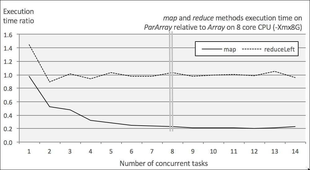
Impact of concurrent tasks on the performance on Scala parallelized map and reduce

The test executes the mapper and reducer functions 1 million times on an 8-core CPU with 8 GB of available memory on JVM.

The results are not surprising in the following respects:

The second test consists of comparing the behavior of two parallel collections, ParArray and ParHashMap, on two methods, map and filter, using a configuration identical to the first test as follows:

val sz = 10000000
val mData = new HashMap[Int, Double]
Range(0, sz).foreach( mData.put(_, nextDouble)) //9
val mParData = new ParHashMap[Int, Double]
Range(0, sz).foreach( mParData.put(_, nextDouble))

val bench = new ParallelMap[Double](mData, mParData, times)
Range(1, NTASKS).foreach(bench.map(mapper)(_)) //10
val filterer = (x: Double) => (x > 0.8) 
Range(1, NTASKS).foreach( bench.filter(filterer)(_)) //11

The test initializes a HashMap instance and its parallel counter ParHashMap with 1 million random values (line 9). The benchmark, bench, processes all the elements of these hash maps with the mapper instance introduced in the first test (line 10) and a filtering function, filterer (line 11), with NTASKS = 6. The output is as shown here:

Impact of concurrent tasks on the performance on Scala parallelized array and hash map

The impact of the parallelization of collections is very similar across methods and across collections. The performance of all 4 parallel collections increases 3 to 5 fold as the number of concurrent tasks (threads) increases. It is interesting to notice that the performance of these 4 collections stabilizes for tests with more than 4 tasks. Core parking is partially responsible for this behavior. Core parking disables a few CPU cores in an effort to conserve power, and in the case of a single application, consumes almost all CPU cycles.

Clearly, a four-times increase in performance is nothing to complain about. That being said, parallel collections are limited to single host deployment. If you cannot live with such a restriction and still need a scalable solution, the Actor model provides a blueprint for highly distributed applications.