9

–––––––––––––––––––––––

Modeling and Algorithms for Scalable and Energy-Efficient Execution on Multicore Systems

Dong Li, Dimitrios S. Nikolopoulos, and Kirk W. Cameron

9.1   INTRODUCTION

Traditional single microprocessor designs have exerted great effort to increase processor frequency and exploit instruction-level parallelism (ILP) to improve performance. However, they have arrived at a bottleneck wherein doubling the number of transistors in a serial CPU results in only a modest increase in performance with a significant increase in energy. This bottleneck has motivated us into the multicore era. With multicore, we can achieve higher throughput with acceptable power, although the core-level frequency of a multicore processor may be lower than that of a serial CPU. The switch to multicore processors implies widespread in-depth changes to software design and implementation. The popularity of multicore architectures calls for new design considerations for high-performance applications, parallel programming models, operating systems, compiler designs, and so on.

In this chapter, we discuss two topics that are important for high-performance execution on multicore platforms: scalability and power awareness. They are two of the major challenges on multicores [1]. Scalable execution requires efficient resource management. Resource management includes determining the configuration of applications and systems at a given concurrency level, for example, how many tasks should be placed within the same multicore node and how to distribute tasks scheduled into the same node between idle cores. Resource management may also indicate adjusting adaptable frequencies of processors by voltage and frequency settings. Along with an increasing number of nodes and number of processors/cores in highend computing systems, resource management becomes more challenging because the exploration space available for choosing configurations increases explosively. We predict that this resource management problem will be further exacerbated forfuture exascale systems equipped with many-core chips. The explosively increased exploration space requires scalable resource management. To determine the appropriate configurations, we must pinpoint the optimal points in the exploration space without testing every possible configuration. We also must avoid introducing a negative performance impact during the process of configuration determination.

Power-aware execution is the other challenge posed by multicore. Growth in the number of cores of large-scale systems causes continual growth in power. Today, several of the most powerful supercomputers equipped with multicore nodes on the TOP500 List require up to 10 MW of peak power—enough to sustain a city of 40,000 people [2]. The best supercomputer power efficiency is about 0.5‒0.7 Gflops/W [3]. As far as the future exascale systems are concerned, they will require at least 40 Gflops/W to maintain the total cost of ownership, which means two orders of magnitude improvement is needed [3]. With the present trend in power increase, the cost of supplying electrical power will quickly become as large as the initial purchase price of the computing system. High power consumption leads to high utility costs and causes many facilities to reach full capacity sooner than expected. It can even limit performance due to thermal stress on hardware [2].

In this chapter, we study how to create efficient and scalable software control methodologies to improve the performance of high-performance computing (HPC) applications in terms of both execution time and energy. Our work is an attempt to adapt software stacks to emerging multicore systems.

9.2   MODEL-BASED HYBRID MESSAGE-PASSING INTERFACE (MPI)/OPENMP POWER-AWARE COMPUTING

To exploit many cores available on a single chip or a single node with shared memory, programmers tend to use programming models with efficient implementations on cache-coherent shared-memory architectures, such as OpenMP. At the same time, programmers tend to use programming models based on message passing, such as MPI, to execute parallel applications efficiently on clusters of compute nodes with disjoint memories. We expect that hybrid programming models, such as MPI/OpenMP, will become more popular because the current high-end computing systems are scaled to a large amount of nodes, each of which is equipped with processors packing more cores. The hybrid programming models can utilize both shared memory and distributed memory of high-end computing systems.

In this section, we particularly consider hybrid programs that use the common THREAD_MASTERONLY model [4]. Its hierarchical decomposition closely matches most large-scale HPC systems. In this model, a single master thread invokes all MPI communication outside of parallel regions and OpenMP directives parallelize the sequential code of the MPI tasks. Almost all MPI programming environments support the THREAD_MASTERONLY model. This model exploits fast intratask data communication through shared memory via loop-level parallelism. While other mechanisms (e.g., POSIX threads) could add multithreading to MPI tasks, OpenMP supports incremental parallelization and, thus, is widely adopted by hybrid applications. Figure 9.1 depicts a typical iterative hybrid MPI/OpenMP computation, which partitions the computational space into subdomains, with each subdomain handled by one MPI task. The communication phase (MPI operations) exchanges subdomain boundary data or computation results between tasks. Computation phases that are parallelized with OpenMP constructs follow the communication phase. We use the term OpenMP phases for the computation phases delineated by OpenMP parallelization constructs.

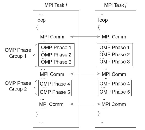
FIGURE 9.1. Simplified typical MPI/OpenMP scheme.

Collections of OpenMP phases delineated by MPI operations form OpenMP phase groups, as shown in Figure 9.1. Typically, MPI collective operations (e.g., MPI_Allreduce and MPI_Barrier) or grouped point-to-point completions (e.g., MPI_Waitall) delineate OpenMP phase groups. No MPI primitives occur within an OpenMP phase group. MPI operations may include slack since the wait times of different tasks can vary due to load imbalance. Based on notions derived from critical path analysis, the critical task is the task upon which all other tasks wait.

Our goal is to adjust configurations of OpenMP phases of hybrid MPI/OpenMP applications by dynamic concurrency throttling (DCT) and dynamic voltage and frequency scaling (DVFS). A configuration includes concurrency configurations and CPU frequency settings. The concurrency configuration specifies how many OpenMP threads to use for a given OpenMP phase and how to map these threads to processors and cores. This can be done by OpenMP mechanisms for controlling the number of threads and by setting the CPU affinity of threads using system calls. We use DCT and DVFS to adjust configurations so as to avoid performance loss while saving as much energy as possible. Also, configuration selection should have negligible overhead. For this selection process, we sample selected hardware events during several iterations in the computation loop for each OpenMP phase and collect timing information for MPI operations. From this data, we build a power-aware performance prediction model that determines configurations that, according to predictions, can improve application-wide energy efficiency.

Table 9.1 Power-Aware MPI /Open MP Model Notation

M	Number of OpenMP phases in an OpenMP phase group
ΔEdctij	Energy saving by DCT during OpenMP phase j of task i
Xij, yij	Number of processors (Xij) and number of cores per processor (yij) used by OpenMP phase j of task i
X, Y	Maximum available number of processors (X) and number of cores (Y) per processor on a node
Tij	Time spent in OpenMP phase j of task i under a confi guration using X processors and Y cores per processor
tij	Time spent in OpenMP phase j of task i after DCT
ti	Total OpenMP phases time in task i after DCT
ti, j, thr	Time spent in OpenMP phase j of task i using a configuration thr with thread count |thr|
N	Number of MPI tasks
f0	Default frequency setting (highest CPU frequency)
Δtijk	Time change after we set frequency fk during phase j of task i

9.2.1   Power-Aware MPI/Open MP Model

Our power-aware performance prediction model estimates the energy savings that DCT and DVFS can provide for hybrid MPI/OpenMP applications. Table 9.1 summarizes the notation of our model. We apply the model at the granularity of OpenMP phase groups. OpenMP phase groups exhibit different energy-saving potential since each group typically encapsulates a different major computational kernel with a specific pattern of parallelism and data accesses. Thus, OpenMP phase groups are an appropriate granularity at which to adjust configurations to improve energy efficiency.

DCT attempts to discover a concurrency configuration for an OpenMP phase group that minimizes overall energy consumption without losing performance. Thus, we prefer configurations that deactivate complete processors in order to maximize the potential energy savings. The energy saving achieved by DCT for task i is

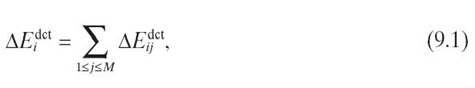
where ΔE_ij^dct is the energy savings for phase j relative to using all cores, when we use x_ij ⋜ X processors and y_ij ⋜ Y cores per processor. If the time for phase j, t_ij, is no longer than the time using all cores T_ij, as we try to enforce, then ΔE_ij^dct ≥ 0 and DCT saves energy without losing performance.

Ideally, DCT selects a configuration for each OpenMP phase that minimizes execution time and, thus, the total computation time in any MPI task. We model this total execution time of OpenMP phases in MPI task i as

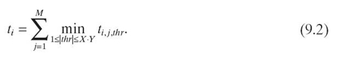
The subscript thr in Equation (9.2) represents a configuration with thread count ∣thr∣.

The critical task has the longest execution time, the critical time, which we model as

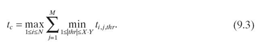
The time difference between the critical task and other (noncritical) tasks in an OpenMP phase group is slack that we can exploit to save energy with DVFS. Specifically, we can use a lower CPU frequency during the OpenMP phases of noncritical tasks. These frequency adjustments do not incur any performance loss if the noncritical task, executed at the adjusted frequencies, does not spend more time inside the OpenMP phase group than the critical time. The slack time that we can disperse to the OpenMP phase group of a noncritical task i by DVFS is

Equation (9.4) reduces the available slack by the DVFS overhead (t_dvfs) and the communication time (t_i^comm_send) for sending data from task i in order to avoid reducing the frequency too much. We depict two slack scenarios for MPI collective operations and MPI_Waitall in. In each scenario, task 0 is the critical task and task 1 disperses its slack to its OpenMP phases.

We select a CPU frequency setting for each OpenMP phase based on the noncritical task´s slack (Δt_i^slack). We discuss how we select the frequency in Section 9.2.3. We ensure that the selected frequency satisfies the following two conditions:

Equation (9.5) sets a time constraint: Δt_ijk refers to the time change after we set the frequency of the core or processor executing task i in phase j to f_k. Equation (9.5) requires that the total time changes of all OpenMP phases at the selected frequencies do not exceed the available slack we want to disperse. Equation (9.6) sets an energy constraint: t_ijk refers to the time taken by phase j of task i running at frequency f_k . We approximate the energy consumption of the phase as the product of time and frequency. Equation (9.6) requires that the energy consumption with the selected frequencies does not exceed the energy consumption at the highest frequency.

Intuitively, energy consumption is related to both time and CPU frequency. Longer time and higher frequency lead to more energy consumption. By computing the product of time and frequency, we capture the effect of both. Empirical observations [5] found average system power is approximately linear in frequency under a certain CPU utilization range. These observations support our estimate since HPC applications usually have very high CPU utilization under different CPU frequencies (e.g., all of our tests have utilization beyond 82.4%, well within the range of a near-linear relationship between frequency and system power).

9.2.2   Time Prediction for Open MP Phases

Our DVFS and DCT control algorithms rely on accurate execution time prediction of OpenMP phases in response to changing either the concurrency configuration or voltage and frequency. Changes in concurrency configuration should satisfy Equation (9.2). Changes in voltage and frequency should satisfy Equations (9.5) and (9.6).

We design a time predictor that extends previous work that only predicted instructions per cycle (IPC) since intranode DCT only requires a rank ordering of configurations [6, 7]. We require time predictions in order to estimate the slack to disperse. We also require time predictions to estimate energy consumption. We use execution samples collected at runtime on specific configurations to predict the time on other untested configurations. From these samples, our predictor learns about each OpenMP phase´s execution properties that impact the time under alternative configurations. The input from the sample configurations consists of elapsed CPU clock cycles and a set of n hardware event rates (e_{(1…n, s)}) observed for the particular phase on the sample configuration s, where the event rate e_{(i, s)} is the number of occurrences of event i divided by the number of elapsed cycles during the execution of configuration s. The event rates capture the utilization of particular hardware resources that represent scalability bottlenecks, thus providing insight into the likely impact of hardware utilization and contention on scalability. The model predicts time on a given target configuration t, which we call Time_t. This time includes the time spent within OpenMP phases plus the parallelization overhead of those phases.

For an arbitrary collection of samples, S, of size ∣S∣, we model Time_t as a linear function:

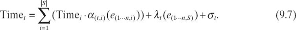
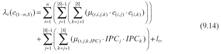
The term λ_t is defined as

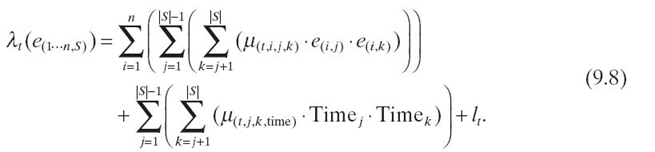
Equation (9.7) illustrates the dependency of terms α_{(t, i)}, λ_t, and σ_t on the target configuration. We model each target configuration t through coefficients that capture the varying effects of hardware utilization at different degrees of concurrency, different mappings of threads to cores, and different frequency levels. The term α_{(t, i)} scales the observed Time_i on the sample configurations up or down based on the observed values of the event rates in that configuration. The constant term σ_t is an event rate-independent term. It includes the overhead time for parallelization or synchronization. The term λ_t combines the products of each event across configurations and of Time_j/k to model interaction effects. Finally, µ is the target configuration specific coefficient for each event pair and l is the event rate-independent term in the model.

We use multivariate linear regression (MLR) to obtain the model coefficients (α, µ, and constant terms) from a set of training benchmarks. We select the training benchmarks empirically to vary properties such as scalability and memory boundedness. The observed time Time_i, the product of the observed time Time_i, and each event rate and the interaction terms on the sample configurations are independent variables for the regression, while Time_t on each target configuration is the dependent variable. We derive sets of coefficients and model each target configuration separately.

We use the event rates for model training and time prediction that best correlate with execution time. We use three sample configurations: One uses the maximum concurrency and frequency, while the other two use configurations with half the concurrency—with different mappings of threads to cores—and the second highest frequency. Thus, we gain insight into utilization of shared caches and memory bandwidth while limiting the number of samples.

We verify the accuracy of our models on systems with three different node architectures. One has four AMD Opteron 8350 quad-core processors. The second has two AMD Opteron 265 dua-core processors. The third has two Intel Xeon E5462 quad-core processors. We present experiments with seven OpenMP benchmarks from the NAS Parallel Benchmarks Suite (v3.1) with CLASS B input. We collect event rates from three sample configurations and make time predictions for OpenMP phase samples in the benchmarks. We then compare the measured time for the OpenMP phases to our predictions. Figure 9.2 shows the cumulative distribution of our prediction accuracy, that is, the total percentage of OpenMP phases with error under the threshold indicated on the x-axis. The results demonstrate the high accuracy of the model in all cases: More than 75% of the samples have less than 10% error.

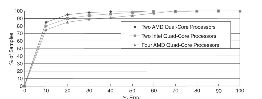
FIGURE 9.2. Cumulative distribution of prediction accuracy.

9.2.3   DCT

With input from samples of hardware event counters collected at runtime, we predict performance for each OpenMP phase under all feasible concurrency configurations based on Section 9.2.2. Intuitively, using the best concurrency configuration for each OpenMP phase should minimize the computation time of each MPI task. We call this DCT strategy the profile-driven static mapping. To explore how well this strategy works in practice, we applied it to the AMG benchmark from the ASC Sequoia Benchmark suite. AMG has four OpenMP phases in the computation loop of its solve phase. Phases 1 and 2 are in phase group 1; phases 3 and 4 are in phase group 2; and the phase groups are separated by MPI_Waitall. We describe AMG in detail in Section 9.2.5. We run these experiments on two nodes, each with four AMD Opteron 8350 quad-core processors.

We first run the benchmark with input parameters P = [2 1 1], n = [512 512 512] under a fixed configuration throughout the execution of all OpenMP phases in all tasks for the entire duration of the run. We then manually select the best concurrency configuration based on these static observations, thus avoiding any prediction errors. The configuration of four processors and two threads per processor, shown as the first bar in each group of bars in Figure 9.3, has the lowest total time in the solve phase and, thus, is the best static mapping that we use as our baseline in the following discussion.

Under this whole-program configuration, each individual OpenMP phase may not use its best concurrency configuration. We select the best configuration for each OpenMP phase and rerun the benchmark, as the second bar in each group of bars in Figure 9.3 shows. We profile each OpenMP phase with this profile-driven static mapping, which we compare with the best static mapping to explore the source of the performance loss. The profiling reveals that three of the four OpenMP phases incur more misses with the profile-driven static mapping, leading to lower overall performance despite using the best configuration based on the fixed configuration runs. This increase arises from frequent configuration changes from one OpenMP phase to another under the profile-driven static mapping.

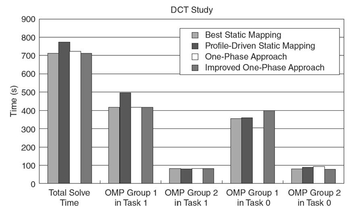
FIGURE 9.3. Impact of different DCT policies on AMG.

Previous work [6] showed that the profile-driven static mapping can outperform the best static mapping. These results combine with ours to demonstrate that the profile-driven static mapping has no performance guarantees: It benefits from improved concurrency configurations while often suffering additional cache misses. We would have to extend our time prediction model to consider the configuration of the previous OpenMP phase in order to capture the impact on cache hit rates. We would also need to train our model under various thread mappings instead of a unique thread mapping throughout the run, which would significantly increase the overhead of our approach.

A simple solution to avoid cache misses caused by changing configurations is to use the same concurrency configuration for all OpenMP phases in each task in isolation. We can predict time for this combined phase and select the configuration that minimizes the time of the combined phase in future iterations under this one-phase approach. Figure 9.3 shows that this strategy greatly reduces the performance loss for AMG compared to the profile-driven static mapping. However, we still incur significant performance loss compared to the best static mapping. Further analysis reveals that the one-phase approach can change the critical task for specific phases despite minimizing the time across all OpenMP phases.

This problem arises because configurations are selected without coordination between tasks. Instead, each task greedily chooses the best configuration for each combined phase regardless of the global impact. To solve this problem, we propose an improved one-phase approach: Each task considers the time at the critical task when making its DCT decision. Each task selects a configuration that does not make its OpenMP phase groups longer than the corresponding ones in the critical task. Although this strategy may result in a configuration where performance for a task is worse than the one achieved with the best static mapping, it maintains performance as long as the OpenMP phase group time is shorter than the corresponding one in the critical task. Unlike the profile-driven static mapping, this strategy has a performance guarantee: It selects configurations that yield overall performance no worse than the best static mapping, as Figure 9.3 shows.

9.2.4   DVFS Control for Energy Saving

Different MPI tasks in a parallel application can have different execution times because of the following: (1) The workload may not be evenly divisible between them; (2) the workload may scale differently in different tasks; (3) heterogeneity of the computing environment; and (4) other system events that may distort execution, such as overheads for the management of parallelism in the runtime system and operating system noise. Any of these events leads to load imbalance, which, in turn, causes slack in one or more MPI tasks. We use DVFS to reduce slack by extending the execution times of OpenMP phases of noncritical tasks, which, in turn, reduces overall energy consumption. More specifically, we use DVFS to select frequencies for the cores that execute each OpenMP phase. We assume for simplicity and to avoid introducing more load imbalance that all cores that execute an OpenMP phase within an MPI task use the same frequency.

We formulate frequency selection as a variant of the 0-1 knapsack problem [8], which is NP-complete. We define the time of each OpenMP phase under a particular core frequency f_k as an item. With each item, we associate a weight, w, which is the time change under frequency f_k compared to using the peak frequency, and a value, p, which is the energy consumption under frequency f_k. The optimization objective is to keep the total weight of all phases under a given limit, which corresponds to the slack time Δt^slack, and to minimize the total value of all phases. Our formulation is a variant of the basic problem since we require that some items cannot be selected together since we assume that we cannot select more than one frequency for eachn OpenMP phase.

Dynamic programming can solve the knapsack problem in pseudopolynomial time. If each item has a distinct value per unit of weight (v = p/w), the empirical complexity is O (log(n))²), where n is the number of items. For convenience in the description of the dynamic programming solution of our variant, we replace p with−p so that we maximize the total value. Let L be the number of CPU frequency levels available and, for OpenMP phase i (0 ≤ i < N, where N is the number of OpenMP phases), let w_{i, j} (1 ≤ j ≤ L) be the available weights associated with CPU frequencies from the lowest to the highest. Let p_{i, j} (1 ≤ j ≤ L) be the available values. The total number of items is n = N × L. The total weight limit is W(i.e., the available slack time). The maximum attainable value with weight less than or equal to Y using items up to j is A(j, Y), which we define recursively as

For the OpenMP phase i,

if ∀ 1 ≤ j <L: w_{i, j} >Y, then

else,

We choose frequencies by calculating A(n, Δt_i^slack)for task i. For a given total weight limit W, the empirical complexity is still O((log(n))²).

9.2.5   Performance Evaluation

We implemented our power-aware MPI/OpenMP system as a runtime library that performs online adaptation of DVFS and DCT. The runtime system predicts execution times of OpenMP phases based on collected hardware event rates and controls the execution of each OpenMP phase in terms of the number of threads, their placement on cores, and the DVFS level. To use our library, we instrument applications with function calls around each adaptable OpenMP phase and selected MPI operations (collectives and MPI_Waitall). This instrumentation is straightforward and could easily be automated using a source code instrumentation tool in combination with a PMPI wrapper library.

In this section, we evaluate our model with two real applications (IRS and AMG) from the ASC Sequoia Benchmark suite.IRS uses a preconditioned conjugate gradient method for inverting a matrix equation. We group its OpenMP phases into four groups. Some OpenMP phase groups include serial code. We regard serial code as a special OpenMP phase with the number of threads fixed to 1. Although DCT is not applicable to serial code, it could be imbalanced between MPI tasks and hence provide opportunities for saving energy through DVFS. We use input parameters NDOMS = 8 and NZONES_PER_DOM_SIDE = 90. The IRS benchmark has load imbalance between the OpenMP phase groups of different tasks. AMG [9] is a parallel algebraic multigrid solver for linear systems on unstructured grids. Its driver builds linear systems for various three-dimensional problems; we choose a Laplace-type problem (problem parameter set to 2). The driver generates a problem that is well balanced between tasks. We modified the driver to generate a problem with imbalanced load. The load distribution ratio between pairs of MPI tasks in this new version is 0.45: 0.55. Figure 9.4 and 9.5 show simplified computational kernels for IRS and AMG.

We deploy our tests in large scales in order to investigate how our model reacts as the number of nodes changes. The following experiments consider the power-awareness scalability of HPC applications, which we call the scalability of energy saving opportunities. We present results from experiments on the System G supercomputer at Virginia Tech. System G is a unique research platform for Green HPC, with thousands of power and thermal sensors. System G has 320 nodes powered by Mac Pro computers, each with two quad-core Xeon processors. Each processor has two frequency settings for DVFS. The nodes are connected by Infiniband (40 Gb/s). We vary the number of nodes and study how our power-aware model performs under strong and weak scaling. We use the execution under the configuration using two processors and four cores per processor and running at the highest processor frequency, which we refer to as (2, 4), as the baseline by which we normalize reported times and energy.

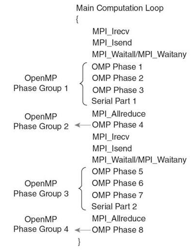
FIGURE 9.4. Simplified IRS flow graph.

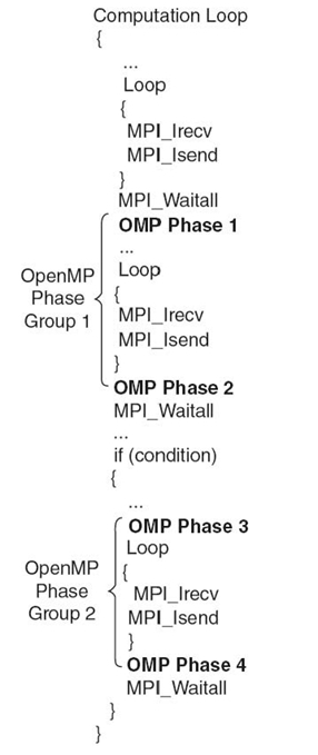
FIGURE 9.5. Simplified AMG flow graph.

Figure 9.6 displays the results of AMG and IRS under strong scaling input (i.e., maintaining the same total problem size across all scales). Actual execution time is shown above normalized execution time bars to illustrate how the benchmark scales with the number of nodes. On our cluster, the OpenMP phases in AMG scale well, and hence DCT does not find energy-saving opportunities in almost all cases, although with 64 nodes or more, DCT leads to concurrency throttling on some nodes. However, due to the small length of OpenMP phases at this scale, DCT does not lead to significant energy savings. When the number of nodes reaches 128, the per-node workload in OpenMP phases is further reduced to a point where some phases become shorter than our DCT minimum phase granularity threshold, and DCT simply ignores them. On the other hand, our DVFS strategy saves significant energy in most cases. However, as the number of nodes increases, the ratio of energy saving decreases from 3.72% (4 nodes) to 0.121% (64 nodes) because the load difference between tasks becomes smaller as the number of nodes increases. With 128 nodes, load imbalance is actually less than DVFS overhead, so DVFS becomes ineffective. In IRS, our DCT strategy leads to significant energy saving when the number of nodes is more than eight. We even observe performance gains by DCT when the number of nodes reaches 16. However, DCT does not lead to energy saving in the case of 128 nodes for similar reasons to AMG.DVFS leads to energy saving with less than 16 nodes but does not provide benefits as the number of nodes becomes large and the imbalance becomes small.

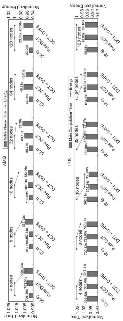
FIGURE 9.6. Results from strong scaling tests of our adaptive DCT/DVFS control on System G

Figure 9.7 displays the weak scaling results. We adjust the input parameters (AMG and IRS) or change the input problem definition (BT- MZ) as we vary the number of nodes so that the problem size per node remains constant (or close to it). For IRS and BT-MZ, the energy-saving ratio grows slightly as we increase the number of nodes (from 1.9% to 2.5% for IRS and from 5.21% to 6.8% for BT-MZ). Slightly increased imbalance, as we increase the problem size, allows additional energy savings. For AMG, we observe that the ratio of energy saving stays almost constant (2.17~2.22%), which is consistent with AMG having good weak scaling. Since the workload per node is stable, energy-saving opportunities are also stable as we vary the number of nodes.

In general, energy-saving opportunities vary with workload characteristics. They become smaller as the number of nodes increases under a fixed total problem size because the subdomain allocated to a single node becomes so small that the energy-saving potential that DVFS or DCT can leverage falls below the threshold that we can exploit. An interesting observation is that, when the number of nodes is below the threshold, some benchmarks (e.g., IRS with less than 16 nodes) present good scalability of energy-saving opportunities for DCT because of the changes in their workload characteristics (e.g., scalability and working data sets) as the allocated subdomain changes. With weak scaling, energy-saving opportunities are usually stable or increasing, and actual energy saving from our model tends to be higher than with strong scaling. Most importantly, under any case, our model can leverage any energy-saving opportunity without significant performance loss as the number of nodes changes.

9.3   POWER-AWARE MPI TASK AGGREGATION PREDICTION

Modern high-end computing systems have many nodes with several processors per node and multiple cores per processor. The distribution of tasks across the cores of multiple nodes impacts both execution time and energy. Current job management systems, which typically rely on a count of available cores for assigning jobs to cores, simply treat parallel job submissions as a two-dimensional (2-D) chart with time along one axis and number of cores along the other [10, 11]. They regard each job as a rectangle with width equal to the number of cores requested by the job and height equal to the estimated job execution time. Most scheduling strategies are based on this model, which has been extensively studied [12, 13]. Unfortunately, these job schedulers ignore the power-performance implications of the layouts of cores available in compute nodes to execute tasks from parallel jobs.

In the previous section, we assume one MPI task per node without consideration of task distribution. In this section, we remove this assumption and consider the effects of task distribution. In particular, we propose power-aware task aggregation.

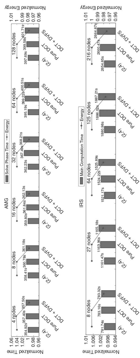
FIGURE 9.7. Results from weak scaling tests of our adaptive DCT/DVFS control on System G

Task aggregation refers to aggregating multiple tasks within a node with shared memory. A fixed number of tasks can be distributed across a variable number of nodes using different degrees of task aggregation per node. Aggregated tasks share system resources, such as the memory hierarchy and network interface, which has an impact on performance. This impact may be destructive because of contention for resources. However, it may also be constructive. For example, an application can benefit from the low latency and high bandwidth of intranode communication through shared memory. Although earlier work has studied the performance implications of communication through shared memory in MPI programs [14, 15], the problem of selecting the best distribution and aggregation of a fixed number of tasks has been left largely to ad hoc solutions.

Task aggregation significantly impacts energy consumption. A job uses fewer nodes with a higher degree of task aggregation. Unused nodes can be set to a deep low-power state while idling. At the same time, aggregating more tasks per node implies that more cores will be active running tasks on the node, while memory occupancy and link traffic will also increase. Therefore, aggregation tends to increase the power consumption of active nodes. In summary, task aggregation has complex implications on both performance and energy. Job schedulers should consider these implications in order to optimize energy-related metrics while meeting performance constraints.

We target the problem of how to distribute MPI tasks between and within nodes in order to minimize execution time, or minimize energy, under a given performance constraint. The solution must make two decisions: how many tasks to aggregate per node; and how to assign the tasks scheduled on the same node to cores, which determines how these tasks will share hardware components such as caches, network resources, and memory bandwidth. In all cases, we select a task aggregation pattern based on performance predictions.

  We assume the following:

• The number of MPI tasks is given and fixed throughout the execution of the application.
• The number of nodes used to execute the application and the number of tasks per node is decided at job submission time, and this decision depends on a prediction of the impact of different aggregation patterns on performance and energy.
• Any aggregation must assign the same number of tasks to each node.
• Jobs are single-program, multiple-data (SPMD) programs.
• MPI communication patterns—including message size and communication target—can vary across tasks.
• Aggregation patterns must not result in total DRAM requirements that exceed a node´s physical memory.

Allowing aggregation patterns that place more tasks on some nodes than others may be more efficient in imbalanced applications; however, the resulting load imbalance would hurt performance and waste energy in well-balanced SPMD applications. In these cases, the system could leverage slack to save energy. We studied energy-saving opportunities due to slack in the previous section.

We decompose the aggregation problem into three subproblems: predicting the impact of task count per node on computation, predicting the communication cost of all aggregation patterns, and combining the computation and communication predictions. We study the impact of aggregation on computation and communication separately since the same aggregation pattern can impact computation and communication differently. Our test platform is a cluster with 16 nodes, each of which has two quad-core processors. The possible aggregation patterns on our platform are shown in Figure 9.8. These aggregation patterns are used throughout this section.

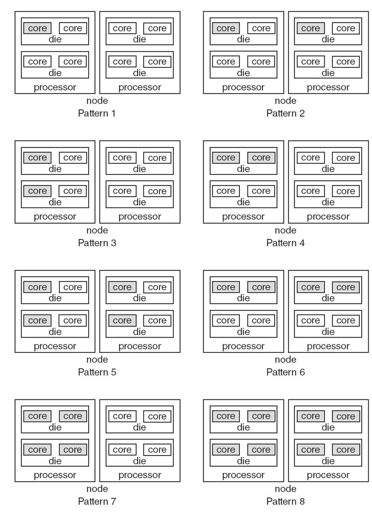
FIGURE 9.8. Aggregation patterns on our test platform.

9.3.1  Predicting Computation Performance

We predict performance during computation phases by predicting IPC. We derive an empirical model based on previous work [6, 7], which predicts the IPC of computation phases in OpenMP applications. We use iteration samples collected at runtime on specific aggregation patterns to predict the IPC for each task on other untested aggregation patterns. The IPC for each aggregation pattern is the average value of the IPC of all tasks. The model methodology is similar to the one in Section 9.2.2. The model derivation is shown in Equation (9.12):

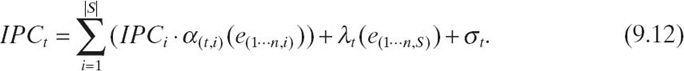
The model predicts the IPC of a specific aggregation pattern t based on information collected in S samples. We collect n hardware event rates e_{(1···n, i)} and IPC_i in each sample i. The function α_{(t, i )}() scales the observed IPC_i in sample i up or down based on the observed values of event rates, while λ_(t) is a function that accounts for the interaction between events and σ_(t) is a constant term for the aggregation pattern t. For a specific sample s, we define α_t as

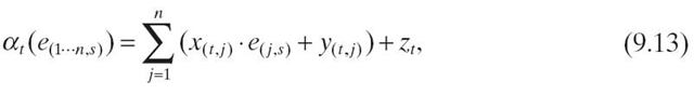
where e_{(j, s)} is a hardware event in simple s, and x_{(t, j)}, y_{(t, j)} and z_t are coefficients. λ_t is defined as

where e_{(j, s)} is the ith event of the jth sample. µ_{(t, i, j, k)}, µ_{(t, i, j, k, IPC)} and l_t are coefficients.

We approximate the coefficients in our model with MLR. IPC, the product of IPC and each event rate, and the interaction terms in the sample aggregation patterns serve as independent variables, while the IPC on each target aggregation pattern serves as the dependent variable. We record IPC and a predefined collection of event rates while executing the computation phases of each training benchmark with all aggregation patterns. We use the hardware event rates that most strongly correlate with the target IPC in the sample aggregation patterns. We develop a model separately for each aggregation pattern and derive sets of coefficients independently. We use the 12 SPEC MPI 2007 benchmarks under different problem sets as training benchmarks. These benchmarks demonstrate wide variation in execution properties such as scalability and memory boundedness.

We classify computation phases into four categories based on their observed IPC during the execution of the sample aggregation patterns and use separate models for different categories in order to improve prediction accuracy. Specifically, we classify phases into four categories with IPC [0, 1), [1, 1.5), [1.5, 2.0), and [2.0, + ∞). Thus, our model is a piecewise linear regression that attempts to describe the relationship between dependent and independent variables more accurately by separately handling phases with low and high scalability characteristics.

We test our model by comparing our predicted IPC with the measured IPC of the computation phases of six NAS MPI parallel benchmarks. Our model is highly accurate with a worst-case absolute error of 2.109%. The average error in all predictions is 1.079% and the standard deviation is 0.7916.

9.3.2   Task Grouping

An aggregation pattern determines how many tasks to place on each node and processor; we must also determine which tasks to collocate. If an aggregation groups k tasks per node and a program uses n tasks, there are ways to group the tasks to achieve the aggregation. For nodes with p ≥ k processors, we then can place the k tasks on one node in ways on the available cores. The grouping of tasks on nodes and their placement on processors has an impact on the performance of MPI point-to-point communication. Computation phases are only sensitive to how tasks are laid out in each node and not to which subset of tasks is aggregated in each node since we assume SPMD applications with balanced workloads between processors. The impact of task placement for MPI collective operations depends on the characteristics of the network; they are relatively insensitive to task placement with flat networks such as fat trees. Thus, we focus on point-to-point operations as we decide which specific MPI ranks to locate on the same node or processor.

Intranode communication has low latency for small messages, while internode high-bandwidth communication is more efficient for large messages because sharing the node´s memory bandwidth between communicating tasks while they exchange large messages incurs sufficient overhead to make it less efficient than internode communication [16]. In addition, the performance of intranode communication is sensitive to how the tasks are laid out within a node: Intranode communication can benefit from cache sharing due to processor die sharing or whole processor sharing. Based on this analysis, we prefer aggregations that group tasks based on whether their communication performance is the best. However, we cannot decide whether to colocate a given pair of tasks based only on individual point-to-point communications between them. Instead, we must consider all communications performed between those tasks and all communications between all tasks. Overall performance may be best even though some (or all) point-to-point communication between two specific tasks is not optimized.

This task grouping problem is an NP-complete problem [17]. We formalize the problem as a graph partitioning problem and use an efficient heuristic algorithm [18] to solve it. We briefly review this algorithm in the following section.

9.3.2.1   Algorithm Review The algorithm partitions a graph G of kn nodes with associated edge costs into k subpartitions, such that the total cost of the edge cut, the edges connecting subpartitions, is minimized. The algorithm starts with an arbitrary partitioning into k sets of size n and then tries to bring the partitioning as close as possible to being pairwise optimal by the repeated application of a two-way partitioning procedure.

The two-way partitioning procedure starts with an arbitrary partitioning {A, B} of a graph G and tries to decrease the initial external cost T (i.e., the total cost of the edge cut) by a series of interchanges of subsets of A and B. The algorithm stops when it cannot find further pairwise improvements. To choose the subsets of A and B, the algorithm first selects two graph nodes a₁, b₁ such that the gain g₁ after interchanging a₁ with b₁ is maximal. The algorithm temporarily sets aside a₁ and b₁ and chooses the pair a₂, b₂ from A−{a₁} and B−{b₁} that maximizes the gain g₂. The algorithm continues until it has exhausted the graph nodes. Then, the algorithm chooses m to maximize the partial sum . The corresponding nodes a₁, a₂,…, a_m and b₁, b₂,…, b_m are exchanged.

9.3.2.2   Applying the Algorithm Task aggregation must group T tasks into n partitions, where n is the number of nodes of a specific aggregation pattern. We regard each MPI task as a graph node and communication between tasks as edges. Aggregating tasks into the same node is equivalent to placing graph nodes into the same partition. We now define an edge cost based on the communication between task pairs.

The original algorithm tries to minimize the total cost of the edge cut. In other words, it tries to place graph nodes with a small edge cost into different partitions. Thus, we must assign a small (large) cost value on an edge that favors internode (intranode) communication. We observe two further edge cost requirements:

• The difference between the small cost value (for internode communication)and the large cost value (for intranode communication) should be large.
• The edge values should form a range that reflects the relative benefit of intra-node communication.

A large difference between edge costs reduces the probability of the heuristic algorithm selecting a poor partitioning. The range of values reflects that colocation benefits some task pairs that communicate frequently more than others.

To assign edge costs, we measure the size of every message between each task pair during execution to obtain a communication table. We then estimate the communication time for each pair of communicating tasks i and j if we place them in the same partition (t_ij^intra) and if we place them in different partitions (t_ij^intra). We estimate these communication times a priori, using a communication benchmark such as MPPtest. Our intranode communication time prediction is conservative since we use the worst-case intranode communication (i.e., two tasks with no processor or die sharing). Finally, we compare t_ij^intra and t_ij^intra to decide whether the tasks i and j benefit from colocation. If t_ij^intra > t_ij^inter, then we set the edge cost to c_ij = 1.0/(t_ij^intra-t_ij^inter). Alternatively, if t_ij^intra ≤ t_ij^inter, we set. These edge costs provide a range of values that reflect the relative benefit of intranode communication as needed.

C is a parameter that ensures the difference of edge costs for pairs of tasks that favor intranode communication and pairs of tasks that favor internode communication is large. We define C as

where k is the number of tasks per node; k² is the maximum number of edge cuts between the two partitions; and Δt is defined as max{1.0/(t_ij^intra-t_ij^inter)}between all task pairs (i, j) that benefit from internode communication.

Overall, our edge costs reflect whether the communication between a task pair is in the intranode or internode communication regime. We apply the graph partitioning algorithm based on these edge costs to group tasks into n nodes. We then use the same algorithm to determine the placement of tasks on processors within a node. Thus, this algorithm calculates a task placement for each aggregation pattern.

9.3.3   Predicting Communication Performance

Modeling and predicting communication time is challenging due to the following reasons:

• computation/communication overlap
• overlap and interference of concurrent communication operations
• even in the absence of overlap, many factors, including task placement (i.e., how MPI tasks are distributed between processors, sockets, and dies in the node), task intensity (i.e., the number of tasks assigned to the node), communication type (i.e., intranode or internode), and communication volume and intensity impact communication interference.

We propose an empirical method to predict a reasonable upper bound for MPI point-to-point communication time.

We trace MPI point-to-point operations to gather the end points of communication operations. We also estimate potential interference based on the proximity of the calls. We use this information to estimate parameters for task placement and task intensity that interfere with each communication operation for each aggregation pattern. Since we predict an upper bound, we assume that the entire MPI latency overlaps with noise from other concurrent communication operations. This assumption is reasonable for well-balanced SPMD applications because of their bulk-synchronous execution pattern.

We construct a prediction table based on our extracted parameters, namely, type of communication (intranode/internode), task intensity, task placement for both communicating and interfering tasks, and message size. We populate the table by running MPI point-to-point communication tests under various combinations of input parameters. We reduce the space that we must consider for the table by considering groups of task placements with small performance difference as symmetric. The symmetric task placements have identical hardware sharing characteristics with respect to observed communication and noise communication.

We use a similar empirical scheme for MPI collectives. However, the problem is simplified since collectives on MPI_COMM_WORLD involve all tasks; we leave extending our framework to handle collective operations on derived communicators as future work. Thus, we only need to test the possible task placements for specific task counts per node for the observed communication.

9.3.4   Choosing an Aggregation Pattern

Our prediction framework allows us to predict the aggregation pattern that either optimizes performance or optimizes energy under a given performance constraint.

We predict the best aggregation pattern based on our computation and communication performance predictions. Since our goal is to minimize energy under a performance constraint, we pick candidates based on their predicted performance and then rank them considering a ranking of their energy consumption.

We predict performance in terms of IPC (Section 9.3.1). To predict performance in terms of time, we measure the number of instructions executed with one aggregation pattern and assume that this number remains constant across aggregation patterns. We verify this assumption by counting the number of instructions under different aggregation patterns for 10 iterations of all NAS MPI parallel benchmarks on a node of our cluster. The maximum variance in the number of instructions executed between different aggregation patterns is negligible (8.5E-05%).

We compare aggregation patterns by measuring their difference to a reference pattern, where there is no aggregation of tasks in a node. We compute the difference as

where t₁^comp, t₁^comm are our estimated computation time and communication time upper bound for the given aggregation pattern, respectively, and t₀^comp, t₀^comm are the computation and communication times for the reference pattern, respectively. Comparing patterns in terms of the difference with a reference pattern partially compensates for the effect of overlap and other errors of time prediction, such as the gap between the actual and predicted communication time. Our analysis in Section 9.3.1 and 9.3.3 estimates performance for each task. For a specific aggregation pattern, Equation (9.16) uses the average computation time of all tasks and the longest communication time.

We choose candidate patterns for aggregation using a threshold of 5% for the performance penalty that any aggregation pattern may introduce when compared to the reference pattern. We discard any aggregation pattern with a higher-performance penalty, which ensures that we select aggregations that minimally impact user experience. An aggregation may actually improve performance; obviously, we consider any such aggregations.

We choose the best aggregation candidate by considering energy consumption. Instead of estimating actual energy consumption, we rank aggregation patterns based on how many nodes, processors, sockets, and dies they use. We rank aggregation patterns that use fewer nodes (more tasks per node) higher. Among aggregation patterns that use the same number of nodes, we prefer aggregation patterns that use fewer processors. Finally, among aggregation patterns that use the same number of nodes and processors per node, we rank aggregation patterns that use fewer dies per processor higher. In the event of a tie, we prefer the aggregation pattern with the better predicted performance. According to this ranking method, the energy ranking of the eight aggregation patterns for our platform in Figure 9.8 from most energy-friendly to least energy-friendly corresponds with their pattern IDs.

9.3.5   Performance

We implemented a tool suite for task aggregation in MPI programs. The suite consists of a PMPI wrapper library that collects communication metadata, an implementation of the graph partitioning algorithm, and a tool to predict computation and communication performance and to choose aggregation patterns. To facilitate collection of hardware event rates for computation phases, we instrument applications with calls to a hardware performance monitoring and sampling library.

We evaluate our framework with the NAS 3.2 MPI Parallel Benchmark suite, using OpenMPI-1.3.2 as the MPI communication library. We present experiments from the System G supercomputer at Virginia Tech.

We set the threshold of performance loss to 5% and use one task per node as the reference aggregation pattern. The choice of the reference aggregation pattern is intuitive since our goal is to demonstrate the potential energy and performance advantages of aggregation, and our reference performs no task aggregation. More specifically, energy consumption is intuitively greatest with one task per node since it uses the maximum number of nodes for a given run. Task aggregation attempts to reduce energy consumption through reduction of the node count. Given that each node consumes a few hundred watts, we will save energy if we can reduce the node count without sacrificing performance. Using one task per node will often improve performance since that choice eliminates destructive interference during computation or communication phases between tasks running on the same node. However, using more than one task per node can improve performance, for example, if tasks exchange data through a shared cache. Since the overall performance impact of aggregation varies with the application, our choice of the reference aggregation pattern enables exploration of the energy-saving potential of various aggregation patterns.

Figure 9.9 shows that our prediction selects the best observed aggregation pattern, namely, the pattern that minimizes energy while not violating the performance constraint, in all cases. We indicate the best observed and predicted task aggregations with stripes. The performance loss threshold is shown with a dotted line. We achieve the maximum energy savings with sp.D.16 (70.03%) and average energy savings of 64.87%. Our prediction of the time difference between aggregation patterns for both computation and communication follows the variance of actual measured time. For FT and BT, we measure performance gains from some aggregation patterns in computation phases and our predictions correctly capture these gains.

The applications exhibit widely varied computation-to-communication ratios, ranging from communication intensive (FT) to computation intensive (LU). The communication time difference across the different aggregation patterns depends on message size and communication frequency. Small messages or less frequent communication result in a smaller communication time difference. For example, 99.98% of the MPI communication operations in lu.D.16 transfer small messages of a size close to 4 kB. The communication time differences in patterns 2‒6 are all less than 10.0%; the communication time differences in patterns 7 and 8 (the most intensive aggregation patterns) are less than 22.7%.

The FT benchmark runs with an input of size 1024 × 512 × 1024 and has MPI_Alltoall operations, in which each task sends 134-MB data to other tasks and receives 134-MB data from other tasks. The communication time differences in patterns 2‒6 range between 28.96% and 144.1%. The communication time difference in pattern 7 (the most intensive aggregation pattern) is as much as 209.7%.

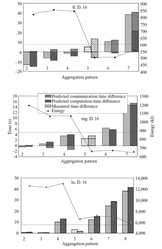
FIGURE 9.9. Results for the NAS 3.2 MPI Parallel Benchmark suite.

We also observe that CG is very sensitive to the aggregation pattern: Different patterns can have significant performance differences due to CG´s memory intensity. Colocating tasks saturate the available memory bandwidth, resulting in significant performance penalties. Finally, we observe MG communication can benefit from task aggregation due to the low latency of communicating through shared memory. In particular, communication time at patterns 2, 3, and 4 reduce by 12.08%, 25.68%, and 48.81%, respectively.

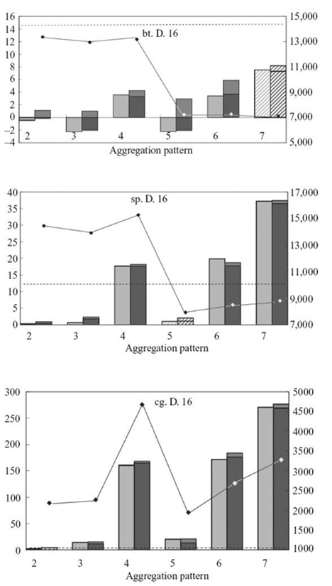
FIGURE 9.9. (Continued)

9.4   CONCLUSIONS

The popularity of multicore architectures demands reconsideration of high-performance application and system designs. Scalable and power-aware execution of parallel applications are two major challenges on multicores. This chapter presents a series of methods and techniques to solve the problems of scalability and energy efficiency for high-end computing systems. We start with research into a power-aware hybrid MPI/OpenMP programming model based on the observation that the hybrid MPI/OpenMP model is gaining popularity. Then, we study power-aware MPI task aggregation, with the goal to improve energy efficiency further. Our power-aware hybrid MPI/OpenMP programming model solves the problem of performance optimization and energy efficiency in a 2-D plane (i.e., DCT + DVFS). We found performance loss when applying DCT at a fine granularity and propose a novel approach to avoid performance loss. To develop a power-aware parallel programming model, we found that the effects of power-saving techniques on local nodes should be considered, as well as the effects on other nodes (i.e., global effects). We introduce task coordination to account for these global effects. We also extend the previous IPC-based DCT performance model to predict execution time based on the requirements of energy estimation and slack time computing. Our scaling study demonstrates that power saving opportunities continue or increase under weak scaling but diminish under strong scaling.

We further research power-aware MPI task aggregation. To predict the impact of task aggregation, we propose a series of methods and techniques. We first predict computation performance. We base our prediction on the information collected from sample aggregation patterns. From this information, we learn execution properties and predict the performance of untested aggregation patterns. We then identify a task grouping problem on which communication performance relies. We formalize the task grouping problem and map it to a classic graph partitioning problem. Given the task grouping, we propose a prediction method based on our analysis of the effects of concurrent intertask communication. We evaluate our methods across different aggregation patterns. Our methods lead to substantial energy saving through aggregation (64.87% on average and up to 70.03%) with tolerable performance loss (under 5%).

REFERENCES

[1] M.F. Curtis-Maury, “Improving the efficiency of parallel applications on multithreaded and multicore systems.” PhD Thesis, Virginia Tech, 2008.

[2] W. Feng and K. Cameron, “The Green500 List: Encouraging sustainable supercomputing,” IEEE Transactions on Computer, 40: 50‒55, 2007.

[3] C. Stunkel, Exascale: Parallelism gone wild! IPDPS Key Note, 2010. Available at http://www.ipdps.org/ipdps2010/ipdps2010-slides/keynote/2010%2004%20TCPP%20 Exascale%20FINAL%20clean.pdf.

[4] R. Rabenseifner and G. Wellein, “Communication and optimization aspects of parallel programming models on hybrid architectures,”International Journal of High Performance Computing Applications, 17: 49‒62, 2002.

[5] T. Horvath and K. Skadron, “Multi-mode energy management for multi-tier server clusters,” in Proceedings of the 17th International Conference on Parallel Architectures and Compilation Techniques (PACT), 2008.

[6] M. Curtis-Maury, F. Blagojevic, C.D. Antonopoulos, and D.S. Nikolopoulos, “Prediction-based power-performance adaptation of multithreaded scientific codes,” IEEE Transactions on Parallel and Distributed Systems (TPDS), 2008.

[7] M. Curtis-Maury, A. Shah, F. Blagojevic, D.S. Nikolopoulos, B.R.de Supinski, and M. Schulz, “Prediction models for multi-dimensional power-performance optimization on many cores,” in Proceedings of the 17th International Conference on Parallel Architectures and Compilation Techniques (PACT), 2008.

[8] M. Silvano and P. Toth, Knapsack Problems: Algorithms and Computer Implementations. New York: John Wiley & Sons, 1990.

[9] H. Van Emden and U.M. Yang, “BoomerAMG: A parallel algebraic multigrid solver and preconditioner,” Applied Numerical Mathematics, 41: 155‒177, 2000.

[10] D.G., Feitelson, L. Rudolph, and U. Schwiegelshohn.“Parallel job schueduling—A status report,”Lecture Notes in Computer Science, 3277: 1‒16, 2005.

[11] S. Srinivasan, R. Keetimuthu, V. Subramani, and P. Sadayappan, “Characterization of backfilling strategies for parallel job scheduling,” in Proceedings of the 2002 International Workshops on Parallel Processing, 2002.

[12] L. Barsanti and A. Sodan, “Adaptive job scheduling via predictive job resource allocation,” Lecture Notes in Computer Science, 4376: 115‒140, 2007.

[13] C.B. Lee and A.E. Snavely, “Precise and realistic utility functions for user-centric performance analysis of schedulers,” in Proceedings of the 16th International Symposium on High Performance Distributed Computing, 2007.

[14] L. Chai, Q. Gao, and D.K. Panda, “Understanding the impact of multi-core architecture in cluster computing: A case study with intel dual-core system,” in The 7th IEEE International Symposium on Cluster Computing and the Grid (CCGrid), 2007.

[15] T. Leng, R. Ali, J. Hsieh, V. Mashayekhi, and R. Rooholamini, “Performance impact of process mapping on small-scale SMP clusters—A case study using high performance linpack,” in Proceedings of the International Parallel and Distributed Processing Symposium (IPDPS), 2002.

[16] D. Li, D.S. Nikolopoulos, K.W. Cameron, B.R.de Supinski, and M. Schulz, “Power-aware MPI task aggregation prediction for high- end computing systems,” in Proceedings of the IEEE Parallel and Distributed Processing Symposium (IPDPS), 2010.

[17] J.M. Orduna, F. Silla, and J. Duato, “On the development of a communication-aware task mapping technique,” Journal of Systems Architecture, 50(4): 207‒220, 2004.

[18] B.W. Kernighan and S. Lin, “An efficient heuristic procedure for partitioning graphs,” Bell System Technical Journal, 49: 291‒308, 1970.