12

–––––––––––––––––––––––

Fault Tolerance and Transmission Reliability in Wireless Networks

Wolfgang W. Bein and Doina Bein

12.1   INTRODUCTION: RELIABILITY ISSUES IN WIRELESS AND SENSOR NETWORKS

With the rapid proliferation of networks, be they wired or wireless, a large number of interconnected devices have been deployed unattended to perform various tasks, ranging from monitoring the nation's critical infrastructure to facilitating civilian applications and business collaborations, to providing intelligence for tactical operations. In the military arena, modern warfare practices mandate the rapid deployment of energy-limited units that stay in constant communication with each other, command centers, and supporting systems such as sensor networks, satellites, and unmanned vehicles. Sensors coupled with integrated circuits, known as “smart sensors,” provide high sensing from their relationship with each other and with higher-level processing layers. Smart sensors find their applications in a wide variety of fields such as military, civilian, biomedical, and control systems. In military applications, sensors can track troop movements and help decide deployment of troops. In civilian applications, sensors can typically be applied to detect pollution, burglary, fire hazards, and the like. Wireless body sensors (called “biosensors”) implanted in the body must be energy-efficient, robust, lightweight, and fault-tolerant, as they are not easily replaceable, repairable, or rechargeable. Biosensors need a dynamic, fault-tolerant network with high reliability. To deliver robust sensor fusion performance, it is important to dynamically control and optimize the available resources. Network resources that are affected by intermittent or permanent disruptions are the sensors and the network capacity. In this chapter, we thus focus on the following: (1) reliable and fault-tolerant placement algorithms, (2) fault-tolerant backbone construction for communication, and (3) minimization of interference by selective adjustment of the transmission range of nodes.

The nodes in a wireless environment are greatly dependent on battery life and power. But if all sensors deployed within a small area are active simultaneously, an excessive amount of energy is used, redundancy is generated, and packet collision can occur. At the same time, if areas are not covered, events can occur without being observed. A density control function is required to ensure that a subset of nodes is active in such a way that coverage and connectivity are maintained. The term “coverage” refers to the total area currently monitored by active sensors; this must include the area required to be covered by the sensor networks. The term “connectivity” refers to the connectivity of the sensor network modeled as a graph. Minimizing the energy usage of the network while keeping its functionality is a major objective in designing a reliable network. But sensors are prone to failures and disconnection. Only minimal coverage of a given region without redundancy would make such a network unattractive from a practical point of view. Therefore, not only is it necessary to design for minimal coverage but also fault-tolerance features must be viewed in light of the additional sensors and energy used. Fault tolerance is a critical issue for sensors deployed in places where they are not easily replaceable, repairable, or rechargeable. Furthermore, the failure of one node should not incapacitate the entire network. As sensor networks have become commonplace, their reliability and fault tolerance, as well as redundancy and energy efficiency, are increasingly important.

Network communication (wired or wireless) is frequently affected by link or node crashes, temporary failure, congestion (wired), and bandwidth. In an ad hoc environment, the set of immediate or nearer neighbors can change at arbitrary moments of time. In sensor networks, the battery determines the lifetime of a node; a node failure can occur frequently as the node becomes older. Thus, in order to increase the throughput on routing the packets, nodes should use fewer routes (a so-called communication backbone of a network). At the same time, since in an ad hoc or sensor network a node can fail or move somewhere else with high frequency, the selected nodes must be provided with enough redundancy for communication. This is done by them acting as alternative routers, and alternative routes have to be available before crashes affect the communication backbone. Wireless communication is less stable than wired since it depends on the nodes'power levels (which affect the transmission range of individual nodes), though it is more flexible and has lower cost. In a wireless environment, every node u in the transmission range of another node v can receive messages from v and send them to other nodes outside the range of v. Unlike in the wired environment, bidirectional communication is not guaranteed between any pairs of nodes since their communication range is not fixed and can vary also based on node power.

Started as a Defense Advanced Research Projects Agency (DARPA) project, the Sensor Information Technology (SensIT) program focused on decentralized, highly redundant networks to be used in various aspects of daily life. The nodes in sensor networks are usually deployed for specific tasks: surveillance, reconnaissance, disaster relief operations, medical assistance, and the like. Increasing computing and wireless communication capabilities will expand the role of the sensors from mere information dissemination to more demanding tasks such as sensor fusion, classification, and collaborative target tracking. The sensor nodes are generally densely scattered in a sensor field, and there are one or more nodes called sinks (or also initiators), capable of communicating with higher-level networks (Internet, satellites, etc.) or applications. By a dense deployment of sensor nodes, we mean that the nearest neighbor is at a distance much smaller than the transmission range of the node.

In general, a spatial distribution of the sensors is a two-dimensional (2-D) Poisson process. The nodes must coordinate to exploit the redundancy provided when they are densely deployed, to minimize the total energy consumption—thus extending the lifetime of the system overall—and to avoid collisions. Selecting fewer nodes saves energy, but the distance between neighboring active nodes could be too large; thus, the packet loss rate could be so large that the energy required for transmission becomes prohibitive. Energy can be wasted by selecting more nodes, and shared channels will be congested with redundant messages; thus, collision and, subsequently, loss of packets can occur. Therefore, minimizing communication cost incurred in answering a query in a sensor network will result in longer-lasting sensor networks. Communication-efficient execution of queries in a sensor network is of significant interest. Wireless sensor networks provide target sensing, data collection, information manipulation, and dissemination in a single integrated framework. Due to the geographical distribution of sensors in a sensor network, each piece of data generated in a sensor network has a geographic location associated with it in addition to a time stamp. Hence, to specify the data of interest over which query should be answered, each query in a sensor network has a time window and a geographical region associated with it. Given a query in a sensor network, we wish to select a small number of sensors that are sufficient to answer the query accurately and satisfy the conditions of coverage as well as connectivity. Constructing an optimal connected sensor cover for a query enables execution of the query in a very energy-efficient manner as we need to involve only the sensors in the connected sensor cover for processing the query without compromising on its accuracy. When data are sent from one node to the next in a multihop network, there is a chance that a particular packet may be lost, and the odds grow worse as the size of the network increases. When a node sends a packet to a neighboring node and the neighbor has to forward it, the receiving and forwarding processes use energy. The bigger the network, the more nodes that must forward data and the more energy is consumed. The end result is that the network performance degrades. Energy-efficient approaches try to limit the redundancy such that minimum amount of energy is required for fulfilling a certain task. At the same time, redundancy is needed for providing fault tolerance since sensors might be faulty, malfunctioning, or even malicious.

The chapter is organized as follows: Section 12.2 discusses the coverage problem for sensor networks from the fault-tolerance and reliability point of view. We describe two 1-fault-tolerant models, the square and hexagonal, and we compare them with one other, as well as with the minimal coverage model proposed by Zhang and Hou [1]. We describe Markov models for various schemes and give their reliability. Section 12.3 describes schemes to choose a set of nodes called “pivots,” from all the nodes in a network, to reduce routing overhead and excessive broadcast redundancy. Section 12.4 focuses on the energy optimization based on the incremental exploration of the network. We perform one-hop neighborhood exploration, but the work can be generalized to two-hop, three-hop,…up to the diameter of the network (the diameter of a network is the minimum number of hops between any two nodes in the network). We describe various distributed algorithms for self-adjusting the transmission range of nodes in a wireless sensor network. We list a number of open problems and we conclude in Section 12.5.

12.2   RELIABILITY AND FAULT TOLERANCE OF COVERAGE MODELS FOR SENSOR NETWORKS

In this section, we focus on the coverage problem for wireless sensor networks from the fault-tolerance and reliability point of view. We describe two 1-fault-tolerant models, the square and hexagonal. We compare these models with each other and with the minimal coverage model proposed by Zhang and Hou [1], and we give the Markov models for their reliability assuming an exponential time-dependent failure rate.

The section is organized as follows. In Section Section 12.2.1, we present existing work addressing the coverage problem. In Section 12.2.2, we present the two 1-fault coverage models; we compare them among each other and the minimal coverage model in terms of the model efficiency (the area covered versus the portion of the sensors area used for coverage) and the probability for the model to function. In Section 12.2.3, we design the Markov models for the reliability of each coverage scheme assuming an exponential time-dependent failure rate.

12.2.1   Background

Finding a minimum number of sensors needed to cover a certain area and thus finding patterns for wireless sensor networks that are optimal in the sense of coverage are difficult problems, and few results are available in the literature. In the case where both coverage and connectivity are desired, Zhang and Hou [1] have shown that a regular triangular lattice pattern (also known as “uniform sensing range model”) is optimal when the ratio between the communication range and the sensing range, denoted as r_cs, is not greater than . This result can be also found in the work of Kershner [2]. Zhang and Hou [1] also have shown that if the ratio r_cs ≥ 2, then coverage implies connectivity.

For certain fixed values of connectivity, several patterns for coverage have been considered. When a network is sought to have the connectivity of 1, then the strip pattern proposed by Wang et al. [3] was shown by Bai et al. [4] to be asymptotically optimal for any ratio r_cs. For the connectivity of 2, a variant of this strip pattern was shown by Bai et al. [4] to be asymptotically optimal. For such a strip pattern, consider two sensors, a and b, relatively close to each other; that is, the distance between them is larger than the communication range but smaller than twice the communication range. Now if a and b belong to two consecutive strips, say strips 1 and 2, they can have a long communication path, which may be as large as the number of sensors on a strip. Sensors a and b communicate using sensors that are at the left or right end of strip 1 and strip 2. Sensor a sends the packet toward one end (say, the right end) of strip 1, which is forwarded by each sensor on strip 1 in that direction. The sensor placed at the end of strip 1 then sends the packet to another sensor placed between the ends of the two strips. This sensor, in turn, sends it to end of strip 2, and then finally, it is forwarded from right to left toward sensor b. To shorten such a communication path and to achieve 4-connectivity, Bai et al. [5] have used Voronoi polygons and have proposed a diamond pattern that is asymptotically optimal when the ratio r_cs > . If the ratio r_cs≥ , the diamond pattern is the minimal coverage model. If the ratio r_cs < , the diamond pattern is our proposed square model.

Hunag and Tseng [6] have focused on determining whether each point of a target area is covered by at least k sensors. Zhou et al. [7] have extended the problem further and have considered the selection of a minimum size set of sensor nodes that are connected in such a way that each point inside the target area is covered by at least k sensors. Starting from the minimal coverage model, Wu and Yang [8] have proposed two models in which sensors have different sensing ranges. Variable sensing ranges are novel, and in some cases, the proposed models achieve lower energy when energy consumed by the sensor is proportional to the quadratic power of its transmission range. However, both models are worse than the minimal coverage model in terms of achieving better coverage: The ratios of the two proposed models between the area covered and the sum of areas covered by each sensor—we call this ratio the efficiency—are lower than the ratio for the minimal coverage model. Also, the second model proposed in Reference 8 requires (for some sensors) the communication range to be almost four times larger than the sensing range; otherwise, connectivity is not achieved. More precisely, the ratio of the communication range and the coverage range has to be at least .

Delaunay triangulations have been used extensively for wireless networks, especially for topology control of ad hoc networks (see the work of Hu [9]). As well, Voronoi polygons have been used in ad hoc networks for routing boundary coverage and distributed hashing (see the work of Stojmenovic et al. [10‒12]). We also mention that a relay node, also called gateway (Gupta and Younis [13]) or application node (Pan et al. [14]), acts as cluster head in the corresponding cluster. Hao et al. [15] have proposed a fault-tolerant relay node placement scheme for wireless sensor networks and a polynomial time approximation algorithm that selects a set of active nodes, given the set of all the nodes.

Placing the sensors in a network that provides connectivity, coverage, and fault tolerance is of interest in biomedicine. Schwiebert et al. [16] have described how to build a theoretical artificial retina made up of smart sensors, used for reception and transmission in a feedback system. The sensors produce electrical signals that are subsequently converted by the underlying tissue into chemical signals to be sent to the brain. The fault-tolerance aspect of such a network ensures that, in case a sensor fails, there is no immediate need in replacing the sensor or the entire network for the artificial retina to continue its functionality.

12.2.2   Proposed Fault-Tolerant Models

Two parameters are important for a sensor node: the wireless communication range of a sensor, r_C, and the sensing range, r_S. They generally differ in values, and a common assumption is that r_C ≥ r_S. Obviously, two nodes, u and v, whose wireless communication ranges are r_Cu and r_Cv, respectively, can communicate directly if dist(u, v) ≤ min (r_Cu, r_Cv). Zhang and Hou [1] proved that if all the active sensor nodes have the same radio range r_C and the same sensing range r_S, and the radio range is at least twice of the sensing range r_C ≥ 2 × r_S, complete coverage of an area implies connectivity among the nodes. Under this assumption, the connectivity problem reduces to the coverage problem.

There is a trade-off between minimal coverage and fault tolerance. For the same set of sensors, a fault-tolerant model will have a smaller area to cover. Or, given an area to be covered, more sensors will be required, or the same number of sensors but with a higher transmission range. A network is k-fault-tolerant if, by removal of any k nodes, the network preserves its functionality. A k-fault-tolerant network that covers a given region will be able to withstand k removals: By removing any k nodes, the region remains covered. A 0-tolerant network will not function in case some node is removed. To transform a 0-fault-tolerant network into a 1-fault-tolerant network, straightforward approaches are to either double the number of sensors at each point or to double the transmission range of each sensor. Similar actions can be taken to transform a 1-fault-tolerant network into a 2-fault-tolerant one, and so forth.

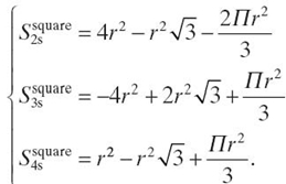
We present first the square 1-fault-tolerant model. The basic structure for this model is composed of four sensors arranged in a square-like shape of side r and is shown in Figure 12.1. A 2-D region of dimension (rN) × (rM), with N and M strictly positive integers, requires (N + 1) × (YM + 1) sensors arranged in this pattern.

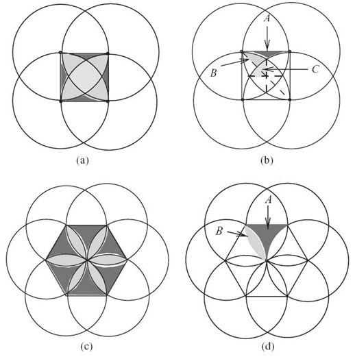
FIGURE 12.1. The square (a, b) and the hexagonal model (c, d).

We partitioned the square surface S₄ = r² into three areas: one area covered by exactly two sensors (S_2s^square), one area covered by exactly three sensors (S_3s^square), and one area covered by exactly four sensors (S_4s^square). To analyze the fault tolerance of such placement, we compute the surface of each such areas. (See Bein et al. [17] for a discussion of methods.) Let A, B, and C be the disjoint areas as drawn in Figure 12.1. We observe that S_2s^square = 4S_A, S_3s^square = 8S_B, and S_4s^square = 4S_C, and we obtain that

Therefore, given a 2-D region of dimension (rN) × (rM), the ratio between the sensor area used and the area covered is

.

The area covered by two sensors is

.

The area covered by three sensors is

.

The area covered by four sensors is

.

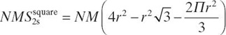
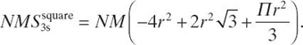
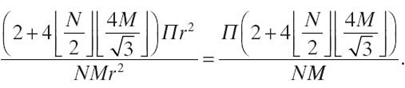
A similar analysis can be done for the hexagonal 1-fault-tolerant model. The basic structure for this model is composed of six sensors arranged in a regular hexagon-like shape of side r and is shown in Figure 12.1. A 2-D region of dimension (rN) × (rM), with N and M strictly positive integers, requires sensors arranged in this pattern.

The hexagonal surface is partitioned into two areas: one area covered by exactly two sensors (S_2s^hexagon) and one area covered by exactly three sensors S_3s^hexagon. To analyze the fault tolerance of such placement, we compute the surface of each such areas. (See also Bein et al. [17].) Let A and B be the disjoint areas as drawn in Figure 12.1. We observe that S_2s^hexagon = 6S_A and S_3s^hexagon = 6S_B, and we obtain that

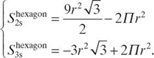
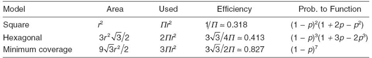
TABLE 12.1. Comparisons among the Models

Given a 2-D region of dimension (rN)×(rM), the ratio between the sensor area used and the area covered is

We compare next the minimal coverage model of Zhang and Hou [1] with the two proposed models in terms of the model efficiency (the area covered versus the portion of the sensors area used for coverage) and the probability for the model to function.

Table 12.1 contains comparative results. We use the following notations. The term area denotes the area covered by the polygonal line formed by the sensors. The term used denotes the portion of the sensor areas used for covering that area. (This value aids in calculating the energy used for covering the region.) This value is obtained by adding for each sensor the portion of its sensor area that covers it. The term efficiency denotes the efficiency of using a particular model and is defined as the ratio between the covered area and the portion used. The term prob. to function denotes the probability for the model to be functional. Assume that all the sensors, independent of their sensing range, have the probability p to fail, 0 ≤ p ≤ 1; thus, the probability to function for the sensor is 1 − p. Also, we assume that any two failures are independent of one another.

The probabilities to function are obtained as follows. In the case of the minimum coverage model, this network functions only if all sensors are functional; the probability in this case is (1 − p)⁷. Thus, the probability to function is

P_min.cov. = (1 − p)⁷.

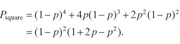
In the case of the square model, this basic network functions if either all sensors are functional (the probability in this case is (1 − p)⁴) or three sensors are functional and one is not (the probability in this case is p(1 − p)³ and is multiplied by the number of such combinations, which is 4), or two diagonally opposed sensors are functional and the other two are not (the probability in this case is p²(1− p)² and is multiplied by the number of such combinations, which is 2). The probability to function is

In case of the hexagonal model, this basic network functions if either all sensors are functional (the probability in this case is (1 − p)⁶) or five sensors are functional and one is not (the probability in this case is p(1 − p)⁵ and is multiplied by the number of such combinations, which is 6), or two nonconsecutive sensors are not functional and the others are (the probability in this case is p²(1 − p)⁴ and is multiplied by the number of such combinations, which is 15), or three nonconsecutive sensors are not functional and the others are (the probability in this case is p³(1 − p)³ and is multiplied by the number of such combinations, which is 2). The probability to function is

P_hexa = (1 − P)⁶ + 6 P (1 − P)⁵ + 15p²(1 − P)⁴ + 2p³(1 − P)³

= (1 − P)²(1 + 3 p + 6 P²-8 P³).

From Table 12.1 we note that the minimal coverage model has the best efficiency, followed by the hexagonal and square model.

As far as the probability to function, the minimal coverage model has the lowest value. For any value of p ∈ [0, 1], the square model is better than the hexagonal.

12.2.3   Reliability Function of the Proposed Models

Reliability is one of the most important attributes of a system. Markov modeling is a widely used analytical technique for complex systems [18‒20]. It uses system state and state transitions. The state of the system comprises all it needs to be known to fully describe it at any given instant of time [18]. Each state of the Markov model is a unique combination of faulty and nonfaulty modules. There is one state called F, which is the failed state (the system does not function anymore). A state transition occurs when one or more modules had failed or had recovered (if possible), and is characterized by probabilities (to fail or to recover).

The exponential failure law states that the reliability of a system varies exponentially as a function of time, for a constant failure rate function. The reliability of the system at time t, R(t), is an exponential function of the failure rate, λ, which is a constant:

R(t) = e^–λt,

where λ is the constant failure rate.

If we assume that each module (in our case, each sensor) in the models we have proposed obeys the exponential failure law and has a constant failure rate of λ, the probability of each module (sensor) being failed at some time t + Δt, given that the module (sensor) was operational at time t, is given by 1 − e^−λΔt . For small values of Δt, the expression reduces to 1 − e^−λΔt ≈ λΔt. In other words, the probability that a sensor will fail within the time period Δt is approximately λΔt.

We make three assumptions that are commonly made in reliability:

1. The system starts with no failures (a perfect state).
2. A failure is permanent: Once a module has failed, it does not recover.
3. There is one failure at a time: Two or more simultaneous failures are seen as sequential ones.

For a generic system state S, let P_S(t) be the probability that the system is in state S at the moment time t. For each state S, the probability of the system being in that state at some time t + Δt depends on the probability that the system was in that state S at time t and on any probability that the system was in another state S′, and it has transitioned from S′ to S.

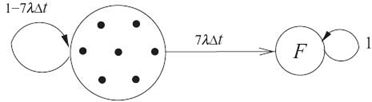
FIGURE 12.2. Markov model of the min. cov. model.

The minimum coverage model is 0-tolerant: The failure of a single node makes the network nonfunctional. The Markov model is shown in Figure 12.2. The single state in which all seven sensors are operational is named “7.” The failed state is named F and is reached when any of the sensors fails. The probability of a sensor to fail within the time interval Δt is λΔt. Thus, the probability of the system to go from state 7 to state F is the probability of any sensor to fail multiplied by the number of such cases, which is 7. The probability of the system to remain in state 7 is 1 minus the probability of the system to go into any other state. Since state F is the only other state reachable from state 7, the probability of the system to remain in state 7 is 1 − 7 λΔt.

The equations of the Markov model of the minimum coverage model can be written from the state diagram shown in Figure 12.2 as follows.

The reliability of the system is the probability of the system to be in any of the nonfailed states R_min.cov.(t) = 1 − P_F(t) = P₇(t). We obtain the system of equations below, with the initial values for P₇(0) = 1 and P_F(0) = 0. Taking the limit as Δt approaches 0 results in a set of differential equations to which Laplace transformation can be applied. Then, we applied the reverse Laplace transformation:

We obtain the reliability of the system to be R_min.cov.(t) = e^−7λt.

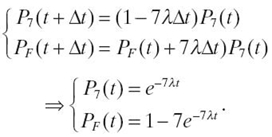
Now for the square fault-tolerant model. The square fault-tolerant model is 1-fault-tolerant: The system is still functional if a single node fails. If two adjacent nodes fail, the system becomes nonfunctional, but if two diagonally opposite nodes fail, the system remains functional. The Markov model of the square fault-tolerant model is shown in Figure 12.3a. It can be reduced further as follows. The single state in which all four sensors are operational is named “4.” The four states in which a single sensor has failed can be reduced to one state named “3.” The two states in which two diagonally opposite sensors have failed can be reduced to one state named “2.” The reduced Markov model is shown in Figure 12.3b.

The reliability of the system is the probability of the system to be in any of the nonfailed states: Rsquare(t) = 1 − P_F(t) = P₄(t) + P₃(t) + P₂(t).

FIGURE 12.3. Square model: Markov model (a) and reduced Markov model (b).

The equations of the Markov model of the square fault-tolerant model can be written from the reduced state diagram shown in Figure 12.3b. Taking the limit as Δt approaches 0 results in a set of differential equations to which Laplace transformation can be applied. Then, we applied the reverse Laplace transformation. We obtain the reliability of the system to be R _square (t) = 2e^−2λt − e^−4λt. (See Reference 17 for more details.)

A similar approach for the hexagonal fault-tolerant model gives a Markov model with more than 30 states. We obtain the reliability of the system to be R_hexagon(t) = 2e^−3λt + 3e^−4λt − 6 e^−5λt + 2e^−6λt. (See also Bein et al. [17].)

12.3   FAULT-TOLERANT_K-FOLD PIVOT ROUTING IN WIRELESS SENSOR NETWORKS

In this section, we describe two schemes to choose a set of nodes called pivots, from all the nodes in a network, in order to reduce the routing overhead and excessive broadcast redundancy.

The section is organized as follows. In Section 12.3.1, we present the problem of backbone construction for a given network and present related work in the literature. In Section 12.3.2, we describe an ordering of nodes based on distance values, the notion of k-fold cover t-set, and the two approximation algorithms for constructing covers.

12.3.1   Background

Current research in wireless networks focuses on networks where nodes themselves are responsible for building and maintaining proper routing (self-configure, self-managing). For all the above reasons, hierarchical structures as dominating sets or a link-cluster architecture are not able to provide sufficiently fast redundancy or fault tolerance for high-speed or real-time networks, where the latency in every node should be very short. The time spent at every node to decide how to route messages should be comparable to the time of the propagation delay between neighboring nodes.

Finding the k-fold dominating set for an arbitrary graph was suggested for the first time by Kratochvil [21]; the problem is -complete (Kratochvil et al. [22]). Liao and Change [23] showed that it is-complete for split graphs (a subclass of chordal graphs) and for bipartite graphs. The particular case k = 1 is, in fact, the minimum dominating set (MDS) problem, and it is -complete for any type of graphs. Approximation algorithms for finding the k-fold dominating set in general graphs were given by Vazirani [24] and Kuhn et al. [25]. The first algorithm for an arbitrary graph of n nodes and the maximum degree of a node Δ by Kuhn et al. [25] runs in O(t²) and gives an approximation ratio of O(tΔ^2/tlog Δ) for some parameter t. The second algorithm, for a unit disk graph, is probabilistic and runs in O(log log n) time, with an O(1) expected approximation. The K-fold dominating set is related to the K-dominating set [26‒28] and to the k-connected k-dominating set [29, 30]. The k-dominating set D ⊆ V has the property that every node in G is not further than k − 1 hops from a node in D. Finding the minimum k-dominating set is -hard, and a number of approximation algorithms are proposed in References 26 and 27. The k-connected k-dominating set has the property that it is k-connected (i.e., by removing at most k − 1 nodes, the graph remains connected, and every node is either in the set or has k immediate neighbors in the set).

The dominating set problem (DS for short) is defined as follows. Given a weighted graph G = (V, E), where each node v ∈ V has associated a weight w_v, and a positive integer m, 0 < m ≤ |V|, find a subset D of size at most m of nodes in V such that every v ∈ V is either in D or has at least one immediate neighbor in D, and the sum is minimized. The corresponding minimization problem is to find the MDS;that is, the size of D is to be minimized. It is approximable within a factor of 1 + log|V| but is not approximable within c for any constant c > 0. Generally, the graph G is considered unweighted (w_v = 1, for all v ∈ V). DS is a particular case of the k-fold dominating set problem defined formally as follows. Given a weighted graph G = (V, E), where each node v ∈ V has associated a weight w_v, and two positive integers k and m, 0 < k ≤ |V| and 0 < m ≤ |V|, find a subset C of size at most m of nodes in V such that every node v ∈ VC has at least k immediate neighbors in C, every node in C has at least k − 1 immediate neighbors in C, and the sum is minimized. We refer to the minimization version of the k-fold dominating set problem as k-fold MDS. Note that MDS is thus a particular case of k-fold MDS, where k = 1. Not every graph has a k-fold dominating set for some arbitrary k; in that case, it is called unfolding.

Obviously, a minimum requirement for a network to have a k-fold dominating set is that k ≤ c, where c is the network connectivity. A graph has connectivity of c if by removing any 1, 2,…, c − 1 nodes, the graph remains connected. A natural way to minimize the number of nodes in the k-fold dominating set is to select not only nodes from the immediate neighborhood but also nodes located at two or more hops. In this way, we do not only have the nodes in the k-fold cover set D act as a backbone for the communication in the network but they can also take on the role of alternative routers for the entire network. Thus, the network can tolerate up to k node failures without losing the routing infrastructure. A k-fold cover t-set (for short, k-fold cover) can be defined as a natural extension of the k-fold dominating set by replacing the term “immediate neighbors” with the term of “nearer neighbors.” Given a fixed parameter t, every node v gathers information about its t nearest neighbors (in terms of distance)—the set called the t-ball of v, B_v (Eilam et al. [31]). A set D ⊆ V is a k-fold cover t-set if, for any node v, |D ∩ B_v| ≥ k (D contains at least k nodes from any t-ball in the network). The elements of D are called pivots .

There is a trade-off between selecting a smaller set of nodes and the power consumption of the selected nodes. Maintaining the routing infrastructure to only a subset of nodes reduces the routing overhead and excessive broadcast redundancy. At the same time, to save energy, unused nonbackbone nodes can go into a sleeping mode and wake up only when they have to forward data or have selected themselves in the k-fold cover set due to failure or movement of nodes. Selecting fewer nodes to act as routers has a power consumption disadvantage: The routers will deplete their power faster than the nonrouter nodes. Thus, once the power level of these nodes falls below a certain threshold, those nodes can be excluded as routers, and some other nodes have to replace them.

Two particular cases of the DS problem are the connected dominating set and the weakly connected dominating set. The connected dominating set problem requires the set of nodes selected as the dominating set to form a connected subgraph of the original graph. The weakly connected dominating set problem, defined by Dunbar et al. [32], requires the subgraph induced by the nodes in the set and their immediate neighbors to form a connected subgraph of the original graph.

12.3.2   Distributed k-Fold Pivot t-Set

A wireless network, which is a point-to-point communication network, is modeled as a connected, weighted, finite digraph G = (V, E, w) that does not contain multi-arcs or self-loops. The set of processors in the network have unique identification (ID) and they are represented by a set of nodes V, |V| = n. We assume that the unique IDs are a contiguous set {1,…, n}. Note that the unique ID of nodes induces a total order; thus, for every pair of nodes u, v ∈ V, either u < v or v < u. An arc e = (u, v) ∈ E is a unidirectional communication link that exists if the transmission range of u is large enough for any message sent by u to reach v. Every arc in the network e = (u, v) ∈ E has associated a weight w(e) that represents the cost (energy) spent by u to transmit a message that will reach v. Because of the nonlinear attenuation property for radio signals, the energy consumption for sending is proportional to at least the square of the power of the transmission range. For simplicity, we extend the domain of w to include all pairs of nodes in the network such that, if node v is not within the transmission range of node u, then w (u, v) = ∞.

The wireless channel has a broadcast advantage that distinguishes it from the wired channel. When a node p uses an omnidirectional antenna, every transmission by p can be received by all nodes located within its communication range. This notion is called wireless multicast advantage (WMA). Thus, a single transmission from a node u suffices to reach all neighbors of u. Note that for any pair of nodes u and v, w(u, v) is not necessarily equal to w(v, u). Given a simple directed path P in the graph, the length of |P| is the sum of the weights of the arcs of P. The distance dist(u, v) in G is the length of the shortest path. For every node v, we can order the rest of the nodes in the digraph G with respect to their distance from v, breaking ties by increasing node ID (Eilam et al. [31]): Formally, x < _vy if and only if dist(x, v) < dist(y, v) or dist(x, v) = dist(y, v) and x < y. The t-ball of node v, B_v(t), is the ordered set of the first t nodes according to the total order <_v. We have (Fact 2.1 from Eilam et al. [31]): If u ∈ B_v(t), then for every node x on the shortest path from v to u, u ∈ B_x(t).

Definition 12.1   Consider a collection of subsets of size t of elements from the node set V. Each subset represents the t closest neighbors (in terms of distance) for some node v in V.

Given a parameter k, k > 0, a set D is a k-fold cover t-set for the collection , or k -fold cover for short, if for every , D contains at least k elements fromB, we write |B ∩ D| ≥ k.

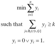
The problem of finding the minimum size k-fold cover set can be modeled as a linear program. Let y_i ∈ {0, 1} be a binary variable associated with some node i ∈ {1,…, n} such that y_i = 1 iff node i is in the k-fold cover. The goal is to minimize the sum of all y variables such that in every t-ball of some node i, there are at least k nodes from the k-fold cover, including node i if i is in the cover. In other words, nodes not in the k-fold dominating set have to be covered at least k times, and nodes in the k-fold dominating set have to be covered at least k − 1 times. The linear program follows:

Next, we present two techniques to approximate a solution for the minimum k-fold cover; one uses a greedy method to select these nodes (so-called pivots), while the second one uses randomization to select them.

Computing the minimum size k-fold cover for any k ≥ 1 is -complete. We extend the two techniques from Awerbuch et al. [33] to generate relatively small k-fold covers for a given collection of sets of a given fixed size t. The first technique (Algorithm Cover 1) uses a greedy approach to select the nodes. The second technique (Algorithm Cover 2) selects each node with a certain probability.

Algorithm Cover 1 starts with the set D to be initially ∅ and iteratively adds to D an element in V occurring in the most uncovered sets. A set is covered if it contains at least k elements, which are also in D. The set D is then called a greedy k-fold cover for C. As in Reference 25, the algorithm to be described uses a coloring mechanism (variable c_i of some node i) to distinguish between two types of nodes: (1) gray color for nodes that are not in the cover and are covered by at least k nodes in the cover, or nodes that are in the cover and are covered by at least k − 1 nodes in the cover, and (2) white color for the nodes that are not in the cover and are not covered by k nodes in the cover, and nodes that are in the cover and are not covered by at least k − 1 nodes in the cover.

Each node in the graph knows the value of n, the total number of nodes in the graph. Besides c_i, a node i uses a variable x_i, which takes discrete values in the set {1/(n − 1), 2/(n − 1),…, (n − 1)/(n − 1)}. Initially, all the nodes are white, D = ∅, and all x-values are 0. Each node i sends a value 1/(n − 1) to all the nodes in its t-ball B_i(T), and the value 0 to the nodes outside its t-ball, excluding itself. There are at most n + 1 rounds (where n = | V |). In round 0, nodes will collect the values received from all the other nodes, and the sum of all the received values is stored in x_i. For some node i, variable x_i has a discrete value from the set {1/(n − 1), 2/(n − 1),…, (n − 1)/(n − 1)}. The larger the value x_i, the higher is the chance for node i to be selected in set D. In round 1, all nodes with x_i = (n − 1)/(n − 1) = 1 announce themselves as pivots and they add themselves to D. Their x-value is already 1. Some white node i receives these messages and stores the IDs of the pivots that are also in its t-ball B_i(t) in variable D_i. If |D_i| ≥ k, then node i changes its color to gray. If, at the end of round 1, there are any white nodes, then the algorithm continues with round 2. In round 2, all nodes with x_i = (n − 2)/(n − 1) announce themselves as pivots, they add themselves to D, and set their x-value to 1. Some white node i receives these messages and adds the IDs of the pivots that are also in its t-ball B_i(t) to variable D_i. If |D_i| ≥ k, then node i changes its color to gray. At the end of round 2, if there are any white nodes, then the algorithm continues with round 3, and so on. If, at the end of round k, 1 ≤ k ≤ n − 1, all nodes are gray, then the algorithm executes the last round, called terminate. In round terminate, all nodes not selected in the k-fold cover (x_i ≠ 1) reset their x-variable to 0.

Lemma 12.1 Let D be a greedy k-fold cover for Then, |D| < |V|·k·(ln|C| + 1)/t.

Algorithm 12.1 Algorithm for Cover1

Actions executed at node i

Initialization (Round 0):

x_i = 0

c_i = white

D_i = ∅

D = ∅

send the value 1/(n − 1) to each node in B_i(t) and

the value 0 to each node in (V {i}) B_i(t)

values sent by node j

Round k, 1 ≤ k ≤ n − 1:

if x_i = (n − k)/(n − 1) then

x_i = 1

broadcast the message msg(pivot, i) that node i is a pivot

on receiving msg(pivot, j)

D ← D ∪ { j }

if (j ∈ B_i(t)) then D_i ← D_i ∪ {j}

if (|D_i| ≥ k) ∧ (x_i = 1 ∧ |D_i| ≥ k − 1) then c_i = gray

if all nodes are gray, then terminate

Round terminate

if x_i ≠ 1 then x_i = 0

Proof: If D₁ is a simple, greedy cover for , then (Lovasz [34]).

Selecting an element for a simple cover of corresponds to selecting at most k elements for a k-fold cover. Thus, if D is a greedy k-fold cover for then   ■

Corollary 12.1   If D is a k-fold cover constructed by Algorithm Cover1 for G, then |D| < n·k·(ln n + 1)/t.

Proof: For our collection , (one t-set for each node). Thus, a greedy k-fold cover for G will have at most n·k·(ln n + 1)/t elements.   ■

Given that |D| ≤ n, one can derive some relationships between k and t from Lemma 12.1 and Corollary 12.1. If k is a constant and given that t < n, it follows that t > k(ln n + 1). Conversely, if t is fixed, that is, there is an upper bound on how many other nodes a node can keep track of, then it follows that k < t/(ln n + 1). Furthermore, if D << n, it follows that t >> k (ln n + 1) (when k is fixed) and k << t/(ln n + 1) (when t is fixed), respectively.

For example, consider the network in Figure 12.4 (n = 10). Each node has associated a pair (ID_i, r_i), where ID_i is the unique ID of the node taken from the set {1,…, n}, and r_i is the transmission radius of node i. As a result, the weight of any outgoing arc of i has the same value, which is proportional with r_i². Let and k = 3. Note that the minimum threefold cover is D_opt = {2, 5, 8, 10}. While selecting the t-balls of size 4, ties are broken by node ID. We enumerate the nodes in a t-ball of some node i in nonascending order of its distance with respect to node i. The t-balls for the nodes in the network are B₁ (4) = {9, 2, 5, 10}, B₂ (4) = {3, 4, 8, 5}, B₃(4) = {2, 4, 8, 5}, B₄ (4) = {2, 3, 8, 5}, B₅ (4) = {6, 8, 10, 2}, B₆ (4) = {5, 7, 8, 2}, B₇ (4) = {6, 8, 2, 5}, B₈ (4) = {2, 5, 6, 7}, B₉ (4) = {1, 2, 5, 10}, B₁₀ (4) = {2, 5, 8, 9}.

At the end of round 0, all nodes are white (see Fig. 12.5a) and the x-values are x₁ = 1/9, x₂ = 9/9, x₃ = x₄ = 2/9, x₅ = 9/9, x₆ = 3/9, x₇ = 2/9, x₈ = 7/9, x₉ = y2/9, and x₁₀ = 3/9. In round 1, nodes 2 and 5 are selected in the threefold cover (marked with a cross), and no node becomes gray (see Fig. 12.5b). In round 2, no node is selected. In round 3, node 8 is selected in the threefold cover, and all nodes except 1 and 9 become gray (see Fig. Fig. 12.5c). In rounds 4‒6, no node is selected. In round 7, nodes 6 and 10 are selected, and all the nodes are gray (see Fig. 12.5d). After round terminate executes, the greedy k-fold cover is D = y{2, 5, 6, 8, 10}, which has only one extra node (node 6) compared to the optimum threefold cover D_opt = {2, 5, 8, 10}.

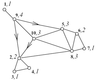
FIGURE 12.4. Network of n = 10 nodes.

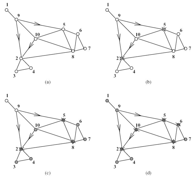
FIGURE 12.5. End of rounds: for round 0 (a), for round 1 (b), for round 3 (c), and for round 7 (d).

Randomization provides yet another method for building the cover. Algorithm Cover 2 simply selects into D each element of V with the probability , for some constant c > 1. D is called a randomized k-fold cover for .

Algorithm 12.2 Algorithm for cover2

Actions executed at node i

With the probability else set x_i = 0

If x_i = 1 then broadcast msg (pivot, i) (node i is a pivot)

Lemma 12.2 Assuming and ln , let D be a randomized k-fold cover for . Then with probability of at least , D is a k-fold cover for and , for some constant C > 1.

Proof: With probability of at least , a randomized, simple cover set D₁ can be constructed for , and the expected size of the constructed cover is |D₁ < , for some constant c > 1 (Awerbuch et al. [33]).

Selecting an element for a simple cover of corresponds to selecting, at most, k elements for a k-fold cover. Thus, with probability of at least , a randomized k-fold cover D can be constructed for , and the expected size of D is      ■

Corollary 12.2   If D is a k-fold cover constructed by Algorithm Cover2 for G, then the expected size of D is |D| < 2·c·n·k·ln n/t, with probability of at least 1 − 1 /1 |C|^c−1, for some constant c > 1.

Proof: For our collection , we have (one t-set for each node). Thus, the expected size of D is |D| < 2·c·n·k·ln n/t, with probability of at least 1 − 1/ n^c−1.      ■

From the definition of k-fold cover set, it can simply be observed that if the degree of some node is smaller than k, the k-fold dominating set has no solution. Thus, the degree of one node can compromise the existence of a k-fold cover set.

But then the k-fold cover set depends less on k and more on t, the number of nodes some node keeps track of. The value of t can vary; it is generally assumed to be more than k. Thus, the k-fold cover set has the advantage that it can be defined for graphs in which the k-fold dominating set cannot be defined. The graph in Figure 12.4 has no threefold dominating set since the degrees of nodes 1, 2, 3, 4, and 7 are less than 3.

On the other hand, if D is a k-fold dominating set for G, then D is also a k-fold cover t-set for G, provided that t ≥ k.

12.4   IMPACT OF VARIABLE TRANSMISSION RANGE IN ALL-WIRELESS NETWORKS

In this section, we focus on developing a communication system optimized for sensor networks that require low power consumption and cost. While the sensor itself requires power, we can design the communication system to use as little power as possible so that the system power will be limited by sensors and not by communication.

The section is organized as follows. In Section 12.4.1, we present work related to reliable communication in wireless sensor networks and the WMA in transmission. In Section 12.4.2, we present the proposed algorithms for adjusting the transmission range (increase or decrease) of selected nodes in the network.

12.4.1   Background

Sankarasubramanian et al. [35] have described wireless sensor networks as event-based systems that rely on the collective effort of several microsensor nodes. Reliable event detection at the sink is based on collective information provided by source nodes and not by any individual report. Conventional end-to-end reliability definitions and solutions are inapplicable in wireless sensor networks. Event-to-sink reliable transport (ESRT) is a novel transport solution developed to achieve reliable event detection in wireless sensor networks with minimum energy expenditure. It includes a congestion control component that serves the dual purpose of achieving reliability and conserving energy. The self-configuring nature of ESRT makes it a robust to random, dynamic topology in wireless sensor networks. It can also accommodate multiple concurrent event occurrences in a wireless sensor field.

Wan et al. [36] have discussed event-driven sensor networks that operate under an idle or light load and then suddenly become active in response to a detected or monitored event. The transport of event pulses is likely to lead to varying degrees of congestion in the network depending on the sensing application. To address this challenge, they proposed an energy-efficient congestion control scheme for sensor networks called congestion detection and avoidance (CODA). Bursty convergecast is proposed by Zhang et al. [37] for multihop wireless networks where a large burst of packets from different locations needs to be transported reliably and in real time to a base station.

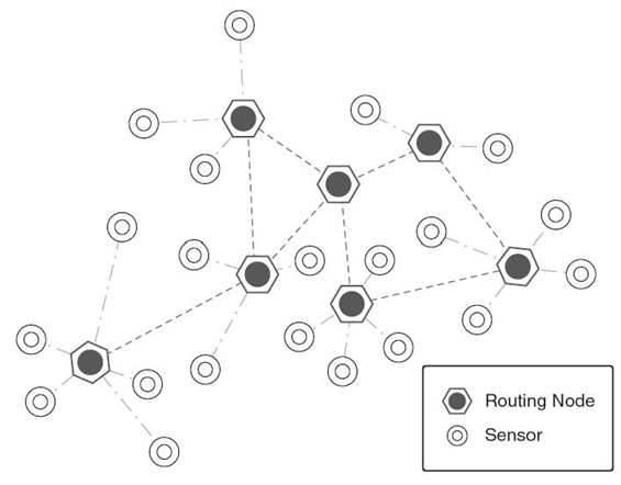
A sensor network is a collection of sensor nodes equipped with sensing, communication (short-range radio) and processing capabilities. Each node in a sensor network is equipped with a radio transceiver or other wireless communication device, and a small microcontroller. The power for each sensor node is derived from a battery. The energy budget for communication is many times more than computation with the available technology. Figure 12.6 depicts a wireless sensor network.

FIGURE 12.6. Routing in WSN.

A sensor will be able to communicate with its neighbors over the shared wireless medium but does not have global knowledge of the entire network. The communication is wireless: for example, radio, infrared, or optical media. Due to the large number of nodes and thus the amount of overhead, the sensor nodes may not have any global ID. In some cases, they may carry a global positioning system (GPS). For most of the wireless sensor networks, nodes are not addressed by their IP addresses but by the data they generate. In order to be able to distinguish between neighbors, nodes may have local unique IDs. Examples of such identifiers are 802.11 MAC addresses [38] and Bluetooth cluster addresses [39].

The neighbors of a sensor are defined as all the sensors within its transmission range. The whole network can be viewed as a dynamic graph with time-varying topology and connectivity. Sensor networks have frequently changing topology: Individual nodes are susceptible to sensor failures. The communications between nodes must be performed in a distributed manner.

Let P_ij be the minimum power necessary for some node i to transmit one message that will reach some other node j in a single hop. The transmission range of node i is the maximum distance to which another node j can be placed such that a single transmission of node i will reach node j. All nodes within the communication range of a transmitting node can receive its transmission (see Fig 12.7). A transmission of power P₁ = P_ij will reach only node j. A transmission of power P₂ = max(P_ij, P_ik) will reach both nodes j and k.

The ability to exploit this property of wireless communication is referred to as WMA. A crucial issue in wireless networks is the trade-off between the “reach” of wireless transmission and the resulting interference by that transmission.

12.4.2   Algorithms

The sensor nodes start arbitrarily with different transmission ranges. The nodes positions are fixed and can adjust the transmission power. However, increasing the transmission power to reach more nodes may consume more energy. Thus, the goal is to reduce the transmission power (i.e., save energy) of a node without disconnecting the node from the rest of the network. By decreasing the transmission range, the distance between various sensors may increase; thus, the diameter of the network may increase. A larger diameter implies a higher chance of interference between the neighboring nodes, while a lower diameter implies a higher chance of message duplication (i.e., the same message will be received twice). When two nodes are not in the communication range of each other, there is a chance that both nodes may send the packets to each other at the same time using the same channel. The nodes will not be able to decide by themselves; hence, a collision will occur. This is known as the hidden terminal problem.

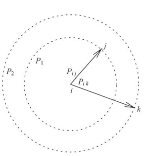
FIGURE 12.7. The wireless multicast advantage.

Let r_i be the transmission range of node i, N_i¹ the one-hop neighborhood of node i, and N_i² the set of nodes situated at no more than two hops. The variables N_i¹ and N_i² are maintained by an underlying local topology maintenance protocol that adjusts its value in case of topological changes in the network due to failures of nodes or links. There are two objectives:

• Objective 1. Reaching more nodes with less increase in power. In the algorithm Adjust_Range, each node will virtually increase its transmission range to reach the current two-hop neighbors. In the algorithm Increase_Range, each node will virtually double its transmission range. For both algorithms, within each neighborhood (i.e., the node and its one-hop neighbors), the node that reaches the most new nodes will be selected to permanently increase its transmission range.
• Objective 2. Reducing the transmission power without losing connectivity in order to save energy. In the algorithm Decrease_Range, within each neighborhood, the node that “loses” the least number of nodes when its transmission range is halved and will not become isolated will be selected.

We are now ready to describe the algorithms. If node i decides to extend its transmission range to reach its two-hop neighbors, node i will be able to acquire more nodes in its new one-hop neighborhood. The cost of this increase is measured in terms of how many new nodes can be reached in one hop by this increase in the transmission range. Assume that every node performs this δ increase. Let N_{i, δ}¹ be the one-hop neighborhood of node i obtained by increasing its transmission range from r_i to r_i + δ. The number of new nodes node i reaches is |N¹_{i, δ}N¹_i|.

Now we describe the algorithm Adjust_Range.

Algorithm 12.3 Adjust_Range

For each node i::

Step 1: Calculate N_i¹.

Step 2: Calculate N_i².

Step 3: Calculate the transmission range r^′_i necessary such that node i will reach its two-hope neighbors.

Calculate the increase in transmission range

Δ r_i = r^′_i – r_i.

Step 4: Calculate the new set of one-hop neighbors NN_i¹ that are obtained by i increasing its transmission range as specified above.

Step 5: Calculate the ratio

FIGURE 12.8. A wireless network.

For all select v_i^∗ that has the highest NR -values.

The one-hope neighbors are N_a¹ = {b, i, j, l}, N_b¹ = {a, c}, N_c¹ = {b, d}, N_d¹ = {c, e}, N_e¹ = {d, f}, N_f¹ = {e, g}, N_g¹ = {f, h l}, N_h¹ = {g, i}, N_i¹ = { a, h}, N_j¹ = {a, k}, N_k¹ = {j}, and N_l¹ = {a}. The two-hope neighbors are N_a² = {c, h, k}, N_b² = {d, i, j, l}, N_c² = {a}, N_d² = {b, f}, N_e² = {c, g}, N_f² = {h}, N_g² = {e, i}, N_h² = {a, f}, N_i² = {b, g}, N_j² = {b, i, l }, N_k² = {a}, and N _l ² = {b, i, j}. Consider the network in Figure 12.8 where the numbers are Euclidean distances between pairs of nodes. Nodes have the following transmission ranges: r_a = 5, r_b = 3, r_c = 2, r_d = 2, r_e = 5, r_f = 5, r_g = 4, r_h = 3, r_i = 2, r_j = 5, r_k = 3, and r_l = 4.

To reach all its two-hop neighbors, a node will alter its transmission range to r′, presented in Table 12.2a. The increase in transmission range Δr and the ratio of increase NR are also presented. In Adjust_Range, the node with the smallest NR-value will be selected to increase its transmission range. For the given example, it is node a. If a node increases its transmission range to reach all its two-hop neighbors, there are cases when other nodes that were at three-hop distance or more will become also reachable. For example, when node a increases its transmission range to reach in one hop its two-hop neighbors, the nodes {d, g} will be now in one-hop range to node a.

The algorithm Increase_Range is described next.

TABLE 12.2. Increasing Transmission Range

Algorithm 12.4  Increase_Range

For each node i::

Step 1: Calculate N_i¹.

Step 2: Double the transmission range r_i′ and calculate the new set of one-hop neighbors DN_i¹ that are obtained by i doubling its transmission range.

Step 3: Calculate the ratio

For all Select v_i^* that has the highest DR-value.

In Figure 12.8, by doubling the transmission ranges, the ratios of increase are presented in Table 12.2b; the ratio of increase DR is also presented. Node a has the smallest DR-value and will be selected to increase its transmission range.

The algorithm Decrease_Range is presented next.

Algorithm 12.5  Decrease_Range

For each node i::

Step 1: Calculate N_i¹.

Step 2: Halve the transmission range and calculate the new set of one-hop neighbors HN_i¹ that are obtained by i halving its transmission range.

Step 3: Calculate the ratio

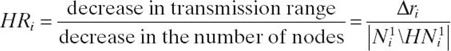
For all v ∈ N_i¹:: Select v* that has the highest HR-value and does not become isolated, HN_i¹ ≠ ∅.

12.5   CONCLUSIONS AND OPEN PROBLEMS

We have proposed two 1-fault-tolerant models, and we have compared them with one another, and with the minimal coverage model expanded to seven nodes instead of three nodes. We note that the minimal coverage model has the best efficiency followed by the hexagonal and the square model. As far as the probability to function, the minimal coverage model has the lowest value. For any value of p ∈ [0, 1], the square model is better than the hexagonal model. The most unreliable model among these models is the minimum coverage model; the square model is more reliable than the hexagonal model. Currently, work is on algorithms to move sensors in order to preserve the network functionality when more than one fault occurs. If the network layout is composed of hundreds of patterns (as proposed here), in some cases, sensors need to be moved to cover areas left uncovered by faulty or moving sensors.

Selecting a small set of nodes among all the nodes in a network, and maintaining the routing infrastructure to only a subset of nodes reduces the routing overhead and excessive broadcast redundancy. Since nodes can maintain shortest paths to a small number of other nodes with limited memory, a simple cover set guarantees coverage but not fault tolerance. (A simple cover set guarantees that every node is “covered” by at least one pivot, the nearest one in terms of distance or weight.) By imposing that every node should be covered by at least k pivots, we guarantee an f-fault-tolerant communication, where f = min(k, c), c being the network connectivity. An important difference between the k-fold MDS and the k-fold cover is that we can extend the range of searching for a pivot. Pivots are not necessarily selected among the immediate neighbors but from a larger neighborhood further away, thus allowing smaller subsets and a better chance of stability when an event affects an entire region of nodes. The relationship between the size of the k-fold cover set and the k-fold dominating set is still open. We conjecture that the size of the k-fold cover set is no greater than the size of the k-fold dominating set.

We name the principles used in the energy optimization method described here on the incremental exploration of the network. We perform one-hop neighborhood exploration, but the principle can be easily generalized to two-hop, three-hop,…up to the diameter of the network. The three algorithms proposed vary the transmission radii of selective sensor nodes to lower the energy spent in broadcasting or the diameter. So, the goal is to reduce the transmission power (i.e., save energy) without reducing the reachability (in terms of the number of nodes). We have proposed algorithms that increase or decrease the transmission range of nodes. Increasing the transmission range of selective nodes will lower the diameter but will increase the total energy. The ratio of the increase in the transmission range to the increase in the number of nodes is calculated for every sensor node, and the node with the smallest ratio will be selected to increase its transmission range. Decreasing the transmission range will lower the total energy but will increase the diameter of the network. Also, a larger diameter implies a higher chance of interference between the neighboring nodes. The ratio of the decrease in the transmission range to the decrease in the number of nodes is calculated for every node, and the node with the highest ratio is selected to decrease its transmission range. Details on variable transmission range beyond the presentation of this book chapter can be found in Reference 40. When two nodes are in not in the communication range of each other, there is a probability that both the nodes send the packets to each other at the same time using the same channel. The nodes will not be able to decide by themselves; hence, a collision will occur (hidden terminal problem). A lower diameter also implies a higher chance of message duplication; that is, the same message will be received twice. Though in our experiments we have modified the transmission range of a single node in the network, we have described our algorithms in terms of selecting nodes from individual neighborhoods. A neighborhood is a node together with its neighbors. Also, experiments were conducted in 2-D Euclidean space. The three algorithms can be applied to graphs using three-dimensional Euclidean metrics. In fact, our algorithms can be applied to general graphs in which the distance between two nodes is an arbitrary positive value.

A venue to be explored in adjusting the transmission range of selective nodes is to apply a load balancing algorithm to either the entire network or to the neighborhood surrounding these selective nodes. It will be interesting to find out whether the structure of the network (e.g., a specific pattern) has influence on the algorithmic procedure of adjusting the transmission range.

REFERENCES

[1] H. Zhang and J.C. Hou, “Maintaining sensing coverage and connectivity in large sensor networks,” in Proceedings of NSF International Workshop on Theoretical and Algorithmic Aspects of Sensor, Ad Hoc Wireless, and Peer-to-Peer Networks, 2004.

[2] R. Kershner, “The number of circles covering a set,” American Journal of Mathematics, 61: 665‒671, 1939.

[3] Y. Wang, C. Hu, and Y. Tseng, “Efficient deployment algorithms for ensuring coverage and connectivity of wireless sensor networks,” in Proceedings of IEEE WICON, pp. 114‒121, 2005.

[4] X. Bai, S. Kumer, D. Xuan, Z. Yun, and T.H. Lai, “Deploying wireless sensors to achieve both coverage and connectivity,” in Proceedings of ACM MOBIHOC, pp. 13‒141, 2006.

[5] X. Bai, Z. Yun, D. Xuan, T.H. Lai, and W. Jia, “Deploying four-connectivity and full coverage wireless sensor networks,” in Proceedings of INFOCOM, pp. 296‒300, 2008.

[6] C.F. Huang and Y.C. Tseng, “The coverage problem in a wireless sensor network,” in ACM International Workshop on Wireless Sensor Networks and Applications (WSNA), pp. 115‒121, 2003.

[7] Z. Zhou, S. Das, and H. Gupta, “Connected k-coverage problem in sensor networks,” in International Conference on Computer Communications and Networks (ICCCN), pp. 373‒378, 2004.

[8] J. Wu and S. Yang, “Coverage issue in sensor networks with ajustable ranges,” in International Conference on Parallel Processing (ICPP), pp. 61‒68, 2004.

[9] L. Hu, “Topology control for multihop packet radio networks,” IEEE Transactions on

[10] I. Stojmenovic, “Voronoi diagram and convex hull based geocasting and routing in wireless networks,” Technical Report TR-99-11, University of Ottawa, 1995.

[11] I. Stojmenovic, A. Ruhil, and D.K. Lobiyal, “Voronoi diagram and convex hull based geocasting and routing in wireless networks,” in Proceedings of IEEE ISCC, pp. 51‒56, 2003.Communications, 41: 1474‒1481, 1993.

[12] I. Stojmenovic, A. Ruhil, and D.K. Lobiyal, “Voronoi diagram and convex hull based geocasting and routing in wireless networks,” Wireless Communications and Mobile Computing, 6 (2): 247‒258, 2006.

[13] G. Gupta and M. Younis, “Fault-tolerant clustering of wireless sensor networks,” in Proceedings of IEEE Wireless Communications and Networking Conference (WCNC), pp. 1579‒1584, 2003.

[14] J. Pan, Y.T. Hou, L. Cai, Y. Shi, and S.X. Shen, “Topology control for wireless sensor networks,” in Proceedings of ACM MOBICOM, pp. 286‒299, 2003.

[15] B. Hao, J. Tang, and G. Xue, “Fault-tolerant relay node placement in wireless sensor networks: Formulation and approximation,” in IEEE Workshop on High Performance Switching and Routing (HPSR), pp. 246‒250, 2004.

[16] L. Schwiebert, S.K.S. Gupta, and J. Weinmann, “Research challenges in wireless networks of biomedical sensors,” in ACM Sigmobile Conference, pp. 151‒165, 2001.

[17] W. Bein, D. Bein, and S. Malladi, “Fault tolerant coverage models for sensor networks,” International Journal of Sensor Networks, 5(4): 199‒209, 2009.

[18] B.W. Johnson, Design and Analysis of Fault-Tolerant Digital Systems. Reading, MA: Addison-Wesley Publishing Company, Inc., 1989.

[19] M.L. Shooman, Probabilistic Reliability: An Engineering Approach. New York: McGraw-Hill, 1968.

[20] K.S. Trivedi, Probability and Statistics with Reliability, Queuing, and Computer Science Applications. Englewood Cliffs, NJ: Prentice-Hall, 1982.

[21] J. Kratochvil, Problems discussed at the workshop on cycles and colourings, 1995. Personal communication.

[22] J. Kratochvil, P. Manuel, M. Miller, and A. Proskurowski, “Disjoint and fold domination in graphs,” Australasian Journal of Combinatorics, 18: 277‒292, 1998.

[23] C.S. Liao and G.J. Change, “k-tuple domination in graphs,” Information Processing Letters, 87: 45‒50, 2003.

[24] V. Vazirani, Approximation Algorithms. Springer: Morgan Kaufmann Publishers, 2001.

[25] F. Kuhn, T. Moscibroda, and R. Wattendorf, “Fault-tolerant clustering in ad hoc and sensor networks,” in Proceedings of the 26th IEEE International Conference on Distributed Computing Systems (ICDCS 06), page 68, 2006.

[26] S. Kutten and D. Peleg, “Fast distributed construction of small k-dominating sets and applications,” Journal of Algorithms, 28: 40‒66, 1998.

[27] L.D. Penso and V.C. Barbosa, “A distributed algorithm to find k-dominating sets,” Discrete Applied Mathematics, 141(1‒3): 243‒253, 2004.

[28] F.H. Wang, J.M. Chang, Y.L. Wang, and S.J. Huang, “Distributed algorithms for finding the unique minimum distance dominating set in split-stars,” Journal of Parallel and Distributed Computing, 63: 481‒487, 2003.

[29] F. Dai and J. Wu, “On constructingk-connected k-dominating set in wireless networks,” in Proceedings of IEEE International Parallel & Distributed Processing Symposium (IPDPS), April 2005.

[30] F. Dai and J. Wu, “On constructing k-connected k-dominating set in wireless ad hoc and sensor networks,” Journal of Parallel and Distributed Computing, 66(7): 947‒958, 2006.

[31] T. Eilam, C. Gavoille, and D. Peleg, “Compact routing schemes with low stretch factor,” in PODC, pp. 11‒20, 1998.

[32] J.E. Dunbar, J.W. Grossman, J.H. Hattingh, S.T. Hedetniemi, and A.A. McRae, “On weakly-connected domination in graphs,” Discrete Mathematics, 168/169: 261‒269, 1997.

[33] B. Awerbuch, A. Bar-Noy, N. Linial, and D. Peleg, “Compact distributed data structures for adaptive routing,” in Symposium on Theory of Computing (STOC), Vol. 2, pp. 230‒240, 1989.

[34] L. Lovasz, “On the ratio of optimal integral and fractional covers,” Discrete Mathematics, 13: 383‒390, 1975.

[35] I. Akyildiz, W. Su, Y. Sankarasubramanian, and E. Cayirci, “A survey on sensor networks,” IEEE Communication Magazine, 42(5): 102‒114, August 2002.

[36] C.Y. Wan, S.B. Eisenman, and A.T. Campbell, “CODA: Congestion detection and avoidance in sensor networks,” in Proceedings of ACM SenSys, pp. 266‒279, 2003.

[37] H. Zhang, A. Arora, Y. Choi, and M. Gouda, “Reliable bursty convergecast in wireless sensor networks,” in Proceedings of ACM MobiHoc, 2005.

[38] IEEE Computer Society LAN MAN Standards Committee, “Wireless lan medium access control (mac) and physical layer (phy) specifications,” Technical Report Tech Report 802.11-1997, Institute of Electrical and Electronics Engineering, New York, 1997.

[39] The Bluetooth Special Interest Group, Bluetooth v1.0b specification, 1999. Available at http://www.bluetooth.com.

[40] D. Bein, A.K. Datta, P. Sajja, and S.Q. Zheng, “Impact of variable transmission range in all-wireless networks,” 42nd Hawaii International Conference in System Sciences (HICSS 2009), 10 pages, 2009.