19

–––––––––––––––––––––––

Maximizing Real-Time System Utilization by Adjusting Task Computation Times

Nasro Min-Allah, Samee Ullah Khan, Yongji Wang, Joanna Kolodziej, and Nasir Ghani

19.1   INTRODUCTION

A real-time system is any information processing system that has to respond to externally generated input stimuli within a finite and specified period: the correctness depends not only on the logical result but also on the time it was delivered; the failure to respond is as bad as the wrong response [1]. Real-time systems can be constructed out of sequential programs but are typically built from concurrent programs called tasks. A real-time task is an executable entity of work that, at a minimum, is characterized by the worst-case execution time (WCET) [2] and time constraints [3]. The WCET is estimated as the maximal time required by the processor to execute the task. A typical timing constraint of a real-time task is the deadline, which is defined as the maximal completion time of a task without causing any damage to the system [4–6].

There are two main classes of real-time systems: (1) hard and (2) soft real-time systems. The hard real-time must meet its deadlines. In case of failure, its operation is without value and the system for which it is a component is of no use. Embedded systems are often hard real-time systems. Such systems have practical applications in tasks or events where strict deadlines are to be followed. In the case where system failure results in a damage or loss of life, the deadlines must be kept [7]. In soft real-time systems, however, there is some room for lateness. A delayed process may not cause the entire system failure. Instead, it may affect the quality of the process or system.

With emergence of many mature scheduling techniques, today the designers of the real-time systems have the freedom to adapt any suitable existing scheduling algorithm that will drive the system efficiently when operational. Therefore, running the time-critical applications with such a scheduling algorithm requires predictable behaviors under all possible circumstances and, hence, mature scheduling techniques need to be adapted. These algorithms are based on system utilization; that is, systems with utilization less than 70% are always schedulable. Developing applications, when the intended workload is fixed, are generally required to fully exhaust the processor capacity when the workload is high or to reduce the energy consumption of the system when the workload is low by reducing operating frequency.

In real-time systems, running the time-critical applications with a scheduling algorithm requires predictable behaviors under all possible circumstances; that is, if a deadline must be missed, it is better to miss the deadline of a less important task than missing the deadline of an important task. Currently, the most commonly used approach to scheduling real-time tasks is priority driven, which falls into two types: fixed priority and dynamic priority [7]. A fixed-priority algorithm assigns the fixed/same priority to all jobs (instances of a task) in each task, which should be different from the priorities assigned to jobs generated by other tasks in the system. In contrast, dynamic-priority scheduling algorithms place no restrictions upon the manner in which priorities are assigned to individual jobs. Although dynamic algorithms are considered better theoretically over fixed-priority techniques, they are difficult to implement in commercial kernels that do not provide explicit support for timing constraints, such as periods and deadlines [8].

Assuming unlimited priority levels, the problem of scheduling periodic tasks under the fixed-priority scheme was first addressed by Liu and Layland [9] in 1973; they derived the optimal static priority scheduling algorithm for an implicit-deadline model (when deadlines coincide with respective periods) called rate monotonic (RM) algorithm. RM assigns static priorities on task activation rates (periods) such that for any two tasks, τ_i and τ_j, priority (τ_i) > priority (τ_j) ⇒ period (τ_i) < period (τ_j), while ties are broken arbitrarily. For a task set with relative deadlines less than or equal to periods (constrained deadline systems), an optimal priority ordering has been shown in Reference 10 to be deadline monotonic (DM), where the priority assigned is inversely proportional to relative deadlines. RM and DM become identical in behaviors when task deadlines and periods are equal. In the last four decades that have followed (since 1973), many of these assumptions are relaxed, and the effects of such changes are highlighted on the monotonic scheduling policy and the corresponding feasibility conditions are provided.

In real-time systems, the system utilization is based on the three basic task parameters, namely, execution time, deadline, and period. Since task periods are usually set by the system requirement as a real-time task has its own periodicity, task deadlines and execution times are the only choices that can be modified in order to improve system utilization. Results are available for modifying the task deadline [11]. Similarly, authors in Reference 12 recently presented a generalized bound for adjusting the task execution times in the context of preemptive RM scheduling policy over uniprocessor systems. In this chapter, we highlight the work of Min-Allah et al. [12] and explain its effectiveness to real-time systems, especially, dynamic voltage scaling (DVS)-enabled systems.

Let Γ = {τ₁, τ₂,…, τ_n} represent a nonconcrete periodic task system having periodic tasks. A nonconcrete periodic task τ_i recurs and is represented by a tuple (c_i, d_i, p_i), where c_i, d_i, p_i represent the WCET, relative deadline, and task period, respectively. Determine whether Γ is RM feasible. There are two possible outcomes: Yes or No. If Γ is feasible, then how much freedom do we have to increase the value of the parameter c_i in order to have a higher system utilization while still satisfying schedulability constraints? If the answer is No (Γ is infeasible), then how is the parameter c_i to be adjusted so that the new task set becomes schedulable?

The application of the aforementioned formulations is enormous, ranging from enhancing quality of service (QoS) to higher system utilization, and so on. A readily available reference is its applicability in a battery-operated embedded system, where DVS is applied to scale down the processor frequency when the processor is not fully loaded [13] for reducing the system energy consumption or increasing system speed for better QoS. The above formulation can be converted into a typical optimization problem concerning the minimization or maximization of a function subject to different types of constraints (equality or inequality) in operation research, which can be solved by any mature algorithm for an efficient solution.

19.2   EXPRESSING TASK SCHEDULABILITY IN POLYLINEAR SURFACES

To find schedulability of a task τ_i, the concept of workload was introduced by the authors of Reference 14. The workload constituted by τ_i at time t consists of its execution demand, c_i, as well as the interference it encounters due to higher-priority tasks from τ_i–1 to τ₁ and can be expressed mathematically as

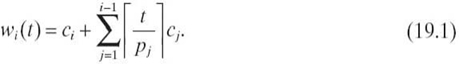
A periodic task τ_i is feasible if we find some t ∈ [0, p_i] satisfying

To check that such a t exists, Equation (19.1) is tested at all points in S_i:

We have the following fundamental theorems to determine whether an individual task and a task set is feasible.

Theorem 19.1 [14]   Given a set of n periodic tasks τ₁,…, τ_n, τ_i can be feasibly scheduled for all task phasings using RM iff

Theorem 19.2 [14]   The entire task set Γ is feasible iff

With Equation (19.3), L_i is needed to be analyzed only at a finite number of points.

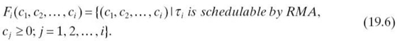
Definition 19.1   F_i [12].The schedulability region F_i is defined as

Definition 19.2   Generalized Bound (P-Bound) [12]. The generalized bound (P-bound) of task τ_i is an inequality g_i(c₁, c₂,…, c_i) ≤ 0 such that

• Any point in the region F_i satisfies g_i(c₁, c₂,…, c_i) ≤ 0.
• Any point that violates g_i(c₁, c₂,…, c_i) > 0 is not in the region F_i.

Definition 19.3  Schedulability Region. According to Definition 19.1, scheduling region F_i that guarantees the schedulability of τ_i is obtained with

Theorem 19.3 [15]   The schedulability region F_i is given by

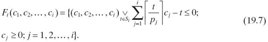
where “∨ ” denotes logic OR and S_i = {rp_j| j = 1,…i; r = 1,…, ⌊p_i /p_j⌋}.

It is observed that Equation (19.7) consists of a set of inequalities with logic OR relations. In the following, a mathematical transformation is proposed to remove logic OR relationships among the inequalities, which enables us to derive the generalized bound.

19.2.1   Generalized Bound/P-Bound

Lemma 19.1 [16]   Let g_i ≤ 0 be a constraint on the schedulability of task τ_i. Suppose g₁ ≤ 0 , g₂ ≤ 0,…, g_m ≤ 0 are constraints with logic OR relationships, then ∀j = 1,…, m, g₁ ≤ 0 ∨ g₂ ≤ 0 ∨ …∨ g_m ≤ 0 can be determined by as a small positive value Δv → 0.

By Lemma 19.1, the constraints with logic OR relationships are turned into one general inequality.

■ EXAMPLE 19.1

Inequalities x ≤ 4 ∨ x ≥ 6 can be determined by

Note that in Lemma 19.1, g₁ = 0 ∨ g₂ = 0 ∨…∨ g_m = 0 is just barely determined by because when Δ v → 0⁺ , we have that ∃j, g_j → 0⁻.

From Lemma 19.1, we have

Theorem 19.4 [12]   The schedulability region F_i can be determined by

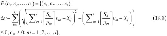
where S_ij is the jth element of S_i, S_i = {rp_j|j = 1,…i; r = 1,…, ⌊p_i /p_j⌋} and k_i is the number of elements in S_i.

19.3   TASK EXECUTION TIME ADJUSTMENT BASED ON THE P-BOUND

The task execution times adjustment problem can be integrated with the P-bound. Say, task periods are fixed and the tasks execution times are kept flexible to improve the system performance. In a very general framework, c_i is the design variable to represent the possible choices of the designer at the stage of the system design; the P-bound is the constraint to ensure the task schedulability; and the objective function is designed as a measure of the overall system performance. Consequently, the problem can be formulated as nonlinear programming optimization problems, which determine the optimum c_i by applying the classical nonlinear optimization approaches.

To make things worse, the time needed to execute these instructions depends on the machine architectures, which is again a complicated activity (the interested reader is referred to References 9, 12, 17, and 18). The point is that, even an estimate on WCET for this simple code is tedious; using loops makes it worst. Assuming a good estimate is made of the source code, there is still uncertainty involved at runtime due to data cache and so on. Another extreme case would be the best-case execution time (BCET). The difference between BCET and WCET can be as large as 80% [19]. The G-bound can be used in this situation by first putting c_i = BCET and then, if the task τ_i is schedulable, the value of c_i can be increased such that c_i = WCET. In case the task is infeasible, the code for τ_i can be readjusted, making WCET lower accordingly. Sometimes, two replicas of the same task can be considered, namely, a primary task and an alternate version of the same task. The primary version has a higher WCET than the alternative one. In such situations, completing either version results in the task being completed. Though the primary version having high quality is desired, the alternative version of the task with acceptable quality may be executed when overload occurs.

The above condition is extended to a more general one by assuming that the execution times c_i(i = 1, 2,…, n) vary within a range; that is, they are described by c_i^min ≤ c_i ≤c_i^max. When feasibility is determined with c_is, there are two possible outcomes: a Yes or a No. The Yes or No answers can be combined into a single optimization problem, which can be formulated formally as follows: Given a set of n periodic tasks Γ = {τ₁, τ₂,…, τ_n}, where the task execution time c_i varies in a range with a lower bound c_i^min and an upper bound c_i^max, and p_i is known a priori, find a set of the execution times c_i under the RM schedulability constraints such that a system performance index is maximized.

Suppose the task system is optimal in the sense that the total processor utilization is maximized. The extended problem can be expressed as a maximization problem:

subject to Equation (19.10), ∀i = 1,…, n,

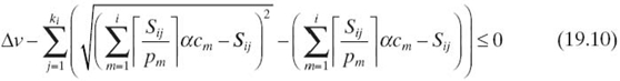
For a given schedulable set, the above maximization problem can be interpreted as computing the minimum processor speed, denoted by α, such that the task set is still schedulable at that speed. Real-time systems are usually battery powered, and the battery is required to be replenished regularly to keep the system operational. These systems generally remain underutilized, and it is recommended to adjust the system speed subject to the workload so that the CPU energy consumption is minimized and the battery life is extended. The speed reduction is considered as scaling the execution times c_i by a factor α. The P-bound for τ_i becomes

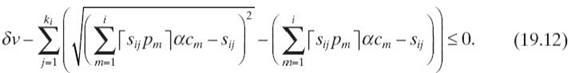
The minimum speed α_min, is given by

The constraints ensure that all the tasks are schedulable. The above maximization problem also is applicable to the cases when an unschedulable task set needs to be converted into a feasible one with the minimum processor speed α, such that the task set becomes schedulable at that speed.

The above maximization formulation allows the systems designer to find the optimal value for the task computation times c_i of a task τ_i within a flexible range, that is, c_i^min ≤ c_i ≤ c_i^max. Any other lower value can result in making the system underutilized, while a higher value can make the system infeasible. Adding α into the feasibility problem determines the lowest possible speed for the system to make it run at the lowest possible feasible speed, hence reducing the overall energy consumption of the system.

19.4   CONCLUSIONS

Real-time applications should remain predictable under all possible circumstances; they should always respect the timing constraints. In this chapter, sensitivity analysis is made for real-time systems and results are applied to sample task sets. It is shown how to use one inequality to express the single task schedulability constraint. The problem of determining the tasks execution times in the space of RM schedulability is solved using optimization techniques. It is concluded that, while designing real-time systems, the P-bound can be directly applied for higher system utilization.

ACKNOWLEDGMENTS

This work is supported by the grand project of the Institute of Software, Chinese Academy of Sciences no. yocx285056, and Higher Education Commission (HEC) of Pakistan under PPCR scheme.

REFERENCES

[1] A. Burns and A. Wellings, Real-Time Systems and Programming Languages. Ada 95, Real-Time Java and Real-Time POSIX, 3rd ed. Boston: Addison Wesley Longman, 2001.

[2] P. Puschner and C. Koza, “Calculating the maximum execution time of real-time programs,” Real-Time Systems, 1(2): 159–176, 1989.

[3] K. Ramamritham, “Where do time constraints come from and where do they go?” International Journal of Database Management, 7(2): 4–10, 1996.

[4] S. Baruah, “Efficient computation of response time bounds for preemptive uniprocessor deadline monotonic scheduling,” Real-Time Systems, 47(6): 517–533, 2011.

[5] P.M. Colom, “Analysis and design of real-time control systems with varying control timing constraints.” PhD Thesis, Automática e Informática Industrial, Barcelona, 2002.

[6] S.U. Khan, S. Zeadally, P. Bouvry, and N. Chilamkurti, “Green networks,” The Journal of Supercomputing, forthcoming.

[7] J.W.S. Liu, Real Time Systems, 1st ed. Upper Saddle River, NJ: Prentice Hall, 2000.

[8] G.C. Buttazzo, “Rate monotonic vs. edf: Judgment day,” Real-Time Systems, 29(1): 5–26, 2005.

[9] H. Aydin, R.G. Melhem, D. Moss, and P. Meja-Alvarez, “Optimal reward-based scheduling for periodic real-time tasks,” IEEE Transactions on Computers, 50(2): 111–130, 2001.

[10] J. Leung and J. Whitehead, “On the complexity of fixed-priority scheduling of periodic,” Performance Evaluation, 2: 237–250, 1982.

[11] N. Min-Allah, X. Jiansheng, and Y. Wang, “Utilization bound for periodic task set with composite-deadline,” Journal of Computers and Electrical Engineering, 36(6): 1101–1109, 2010.

[12] N. Min-Allah, S.U. Khan, and Y. Wang, “Optimal task execution times for periodic tasks using nonlinear constrained optimization,” The Journal of Supercomputing, 59(3): 1120 –1138, 2012.

[13] K. Seth, A. Anantaraman, F. Mueller, and E. Rotenberg, “Fast: Frequency-aware static timing analysis,” Proceedings of the 24th IEEE Real-Time Systems Symposium, pp. 40–51, 2003.

[14] J. Lehoczky, L. Sha, and Y. Ding, “The rate monotonic scheduling algorithm: Exact characterization and average case behavior,” in Proceedings of the IEEE Real-Time System Symposium, pp. 166–171, 1989.

[15] E. Bini and G.C. Buttazzo, “Schedulability analysis of periodic fixed priority systems,” IEEE Transactions on Computers, 53(11): 1462–1473, 2004.

[16] Y. Wang and D.M. Lane, “Solving a generalized constrained optimization problem with both logic and and or relationships by a mathematical transformation and its application to robot path planning,” IEEE Transactions on Systems, Man and Cybernetics, Part C: Application and Reviews, 30(4): 525–536, 2002.

[17] C.M. Krishna and K.G. Shin, Real Time Systems. New York: McGraw-Hill, 1997.

[18] W.K. Shih, J.W.S. Liu, and J.Y. Chung, “Algorithm for scheduing tasks to minimize total error,” SIAM Journal on Computing, 20: 537–552, 1991.

[19] J. Wegener and F. Mueller, “A comparison of static analysis and evolutionary testing for the verification of timing constraints,” Real-Time Systems, 21(3): 241–268, 2001.