
5
–––––––––––––––––––––––
Scalable Computing on Large Heterogeneous CPU / GPU Supercomputers
Fengshun Lu, Kaijun Ren, Junqiang Song, and Jinjun Chen
5.1 INTRODUCTION
Recent advances in the graphics processing unit (GPU) technology have brought enormous benefits to the high-performance computing (HPC) community. Many scientific and engineering applications have achieved order-of-magnitude speedups on energy-efficient CPU/GPU clusters, such as TianHe-1A (TH-1A) [1], Nebulae [2], Lincoln [3] and TSUBAME [4]. Besides the heterogeneity in their processing units, these HPC systems also have complex memory hierarchy: distributed memory across different compute nodes, shared memory within each node, and device memory on GPUs. Consequently, scientific researchers and domain scientists are confronted with great challenges to perform efficient and scalable computing on these heterogeneous HPC infrastructures.
Although most issues of scalable computing on traditional CPU-based HPC systems have been extensively addressed in the past decades [5–9], the scalability issue for newly acknowledged heterogeneous CPU/GPU systems has not been well addressed. We herein give an overview of the recent work on the scalability issue of GPU applications. Goddeke et al. [10] investigated the weak scalability of finite element method (FEM) calculations on a 160-node GPU cluster and observed that the performance of the FEM applications scaled favorably with the number of nodes. Ltaief et al. [11] addressed the challenges in developing scalable algorithms for CPU/GPU platforms and demonstrated that the hybrid Cholesky factorization scaled well with the increasing CPU/GPU couples. Lashuk et al. [12] implemented the fast-multipole method and achieved good weak scalability with the workload of 256 million points on 256 GPUs, which was attributed to the scalable reduction algorithm for the evaluation phase and the data structure transformation tailored for GPU architecture. Jetley et al. [3] scaled the hierarchical N-body simulations on GPU clusters and found that the scalability of applications could be improved by utilizing optimization techniques, such as optimal kernel organization, removal of serial bottlenecks, and workload balance between CPUs and GPUs. Shimokawabe et al. [4] efficiently ported their production weather code to the 528-GPU TSUBAME supercomputer and achieved 80-fold performance over that on a single CPU core. They optimized the boundary-exchange operation by overlapping its communication with the computation to achieve better scalability.
Among the large-scale scientific and engineering applications, there are many legacy programs (such as IFS [13] and WRF [14]) that cannot directly benefit from the immense computational capabilities of heterogeneous HPC systems. It is also impractical to implement them from scratch with other languages like OpenCL [15] or programming paradigms like MapReduce [16]. As such, the ideal approaches are expected not only to preserve most of the legacy code but also to accelerate the computation-intensive kernels on GPUs with vendor-provided programming models. In this chapter, we endeavor to find scalable approaches to make the legacy code benefit from large heterogeneous CPU/GPU systems.
With our approaches, we adopt the existing programming models to construct viable programming patterns targeting large-scale CPU/GPU clusters. We take advantage of the NAS Parallel Benchmark s (NPBs) [17] and a production code for radiation physics in the WRF model to illustrate the strategy of making the legacy code benefited from heterogeneous systems. The remainder of the chapter is organized as follows. Section 5.2 gives a simple overview of the heterogeneous computing environments that include the TH-1A supercomputer and the relevant parallel programming models. Section 5.3 presents our proposed scalable programming patterns for large GPU clusters, which is followed by the detailed hybrid implementations for NPB kernels and RRTM‒LW radiation process in Section 5.4. The experimental results and performance analysis are given in Section 5.5. Finally, Section 5.6 concludes this chapter.
5.2 HETEROGENEOUS COMPUTING ENVIRONMENTS
In this section, we give a short overview of the TH-1A supercomputer and the existing programming models based on which we construct scalable parallel programming patterns for large GPU clusters.
5.2.1 TianHe-1A Supercomputer
The TH-1A supercomputer is built by the National University of Defense Technology and deployed in the National Supercomputing Center in Tianjin. It ranked number 1 in the 36th TOP500 List [18] with maximal Linpack performance of 2.566 PFlops. As depicted in Figure 5.1, TH-1A consists of five subsystems: compute subsystem, service subsystem, storage subsystem, communication subsystem, and the monitoring and diagnosis subsystem. We herein give an emphasis on the compute subsystem and refer the interested readers to References 1 and 19 for more information.
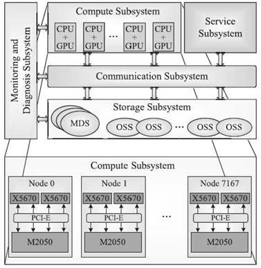
FIGURE 5.1. TH-1A system architecture and the detailed compute subsystem. Adapted from literature [1].
The compute subsystem is constructed with 7168 compute nodes, each of which is configured with two Intel CPUs and one NVIDIA GPU. The CPU is six-core Xeon X5670 (2.93 GHz) and the GPU is Tesla M2050 (1.15 GHz). The peak double-precision performance of each compute node is 655.64 Gflops (i.e., CPU has 140.64 Gflops and GPU has 515 Gflops). The CPUs in compute node fulfill various functionalities, such as running operating systems, managing system resources, and performing general-purpose computation. The GPU mainly executes the computation with abundant data parallelisms in the single-instruction multiple-data (SIMD) scheme. Note that nearly 20% (i.e., 140.64 out of 655.64 Gflops) of the peak performance for each compute node is attributed to the two CPUs. Therefore, efficiently exploiting the computational capacities of both CPUs and GPUs is quite important for HPC on heterogeneous clusters.
5.2.2 Programming Models
Message-passing interface (MPI) [20] provides a standard set of subprogram definitions for implementing parallel programs with a distributed-memory programming model. In the MPI programming model, users manage the communication operations between different MPI processes by calling routines to send and receive messages. In addition, users completely control the workload distribution, which permits the optimization of data locality and workflow. Since it has the advantages of excellent scalability and portability, MPI is an appropriate programming model to accomplish the communication functionality between different compute nodes of large GPU clusters.
OpenMP [21] is an open specification for shared-memory programming. It consists of compiler directives, environment variables, and runtime library routines. Programmers explicitly specify the actions to be taken by the compiler and the runtime system for executing the program in parallel. All OpenMP programs follow the fork-and-join execution model and utilize the work-sharing directives to distribute the workload among the spawned threads. The issues of data dependencies, data conflicts, race conditions, and deadlocks should be addressed by programmers. OpenMP is often used to exploit the fine-grained parallelism of applications on shared-memory architecture.
CUDA [22] is the programming model developed by NVIDIA to harness its powerful GPUs. It has provided support for high-level languages like C/C++ and Fortran, which maintains a low learning curve for programmers. The scientists throughout the industry and academia have already achieved dramatic speedups on production and research applications by utilizing CUDA. In this model, GPU programs are organized into kernels that are performed with abundant threads in the form of thread-blocks. Each thread-block must be scheduled onto one particular streaming multiprocessor (SM), and several thread-blocks may reside on the same SM to hide various latencies. For the devices with compute capability 2.x or higher, programmers can exploit three levels of parallelism within applications, namely, the thread-level, the block-level, and the grid-level parallelism.
5.3 SCALABLE PROGRAMMING PATTERNS FOR LARGE GPU CLUSTERS
Scalable hybrid programming patterns should enable the exploitation of all the computational resources in state-of-the-art GPU clusters, namely, the multicore CPUs and many-core GPUs. CPUs and GPUs can cooperate in the following three ways: (1) CPU accounts for the task of preparing and transferring data and GPU performs arithmetic operations [23]; (2) they perform arithmetic operations from different workloads [24]; and (3) they cooperatively compute the same workload. In this section, we present two hybrid programming patterns and a workload distribution scheme used in the later pattern to ensure the load balance between the CPUs and GPUs.
5.3.1 MPI + CUDA (MC) Hybrid Pattern
The MC pattern depicted in Figure 5.2 has been widely utilized on large clusters based on NVIDIA GPUs [10]. In this hybrid pattern, MPI performs the communication between different nodes of HPC systems and CUDA drives the powerful GPUs. Programs coded under the MC pattern are executed with one MPI process launched on each CPU core, all of which jointly drive the GPU device with CUDA application programming interfaces (APIs).
The latest GPUs support simultaneous execution of kernels from different MPI processes and maintain a separate context for each of these processes. The one-context-per-process scheme inhibits the MPI processes from sharing the objects that reside in the same GPU device. For example, much common data of “state-heavy” geosciences applications can be shared by different MPI processes in the CPU code; however, GPU needs to create data instances for all the MPI processes, resulting in redundant allocations of device memory. Therefore, the problem scale may be bounded by the device memory constraint. Besides, all the MPI processes have to upload data to and download results from GPUs, which inevitably results in many data transfers and exacerbates the memory bandwidth pressure. To address these issues, the MC pattern can be amended by allowing only part of these MPI processes to interact with GPUs and by employing a complicated strategy to ensure the load balance between them.
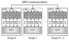
FIGURE 5.2. Schematic diagram for MPI + CUDA parallel programming pattern.
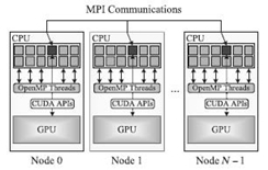
FIGURE 5.3. Schematic diagram for MPI + OpenMP/CUDA parallel programming pattern.
5.3.2 MPI + OpenMP/CUDA (MOC) Hybrid Pattern
We try to address the aforementioned issues by amending the MC pattern with the introduction of OpenMP threads to exploit the parallelism within multicore CPUs.
Figure 5.3 presents another parallel programming model called MOC for large GPU clusters. In this model, only one MPI process is launched on each compute node, which brings two aspects of benefits to state-heavy geosciences applications like WRF. On the one hand, only one context for the MPI process is maintained by GPU and the underutilization of device memory is eliminated. On the other hand, compared with the MC scenario, many fewer data transfers are performed and each one has larger volume, which is favored by GPU devices and can alleviate the memory bandwidth pressure. The MPI process spawns as many OpenMP threads as the amount of CPU cores within each compute node. Only the master thread cooperates with GPU and the others perform relevant arithmetic operations in parallel. Hence, domain experts can exploit the coarse-grained parallelism within applications through MPI and the fine-grained parallelism with OpenMP and CUDA.
Note that the MOC pattern requires a thread-compliant MPI implementation. It should support four thread levels. We mainly focus on the MPI_Thread_Funneled and MPI_Thread_Multiple of them. On the former level, only the master thread can make MPI calls, and all the threads are idle except the master one during the communication process. However, no restrictions exist for the latter level, and multiple threads can call MPI subroutines. When one thread is fulfilling the communication task, other threads can perform computational operations if the task-scheduling scheme is efficiently adjusted [25]. For the sake of simplicity, the MOC pattern only requires the MPI_Thread_Funneled thread-support; otherwise, a complex task-scheduling scheme must be introduced to each application for fully taking advantage of the MPI_Thread_Multiple level.
5.3.3 Workload Distribution Scheme
Assuming that there are M n-core CPUs corresponding to each GPU within a single compute node, the workload assigned to CPUs is accomplished with Mn − 1 CPU cores, leaving one CPU core to interact with GPU. Since CPUs and GPUs have different arithmetic capacities, the key issue for hybrid computing is how to efficiently distribute the workload between these two computing resources. The best workload distribution can be directly obtained by enumerating all the possible distributions and executing the application with each of them. However, that method is rather time-consuming and an efficient workload distribution scheme is highly demanded. In this section, we present an efficient workload distribution scheme for the embarrassingly parallel (EP) applications, which have independent workload and negligible I/O operations.
Let PCPU denote the computing power of each CPU core, then the effective computational capacity of M CPUs and one GPU can be approximated with (Mn − 1) PCPU and PGPU, respectively. Given the workload W, the wall-clock time T for the workload can be shown in Equation (5.1):
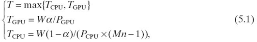
where TCPU(TGPU) denotes the wall-clock time for CPU (GPU) to accomplish the relevant workload, and α represents the workload distribution ratio for GPU. T reaches its minimum at the workload distribution ratio:
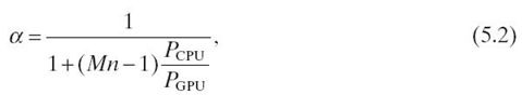
when TCPU is equal to TGPU. Hence, if the relative computing power of CPU over GPU is accurately evaluated, the best workload distribution ratio α can be determined.
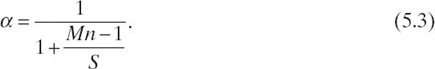
Given the GPU implementation of some particular application, we can obtain its speedup S over the single CPU core counterpart. We substitute PCPU/PGPU of Equation 5.2 with 1/S and get the best workload distribution scheme as
5.4 HYBRID IMPLEMENTATIONS
5.4.1 NAS Parallel Benchmarks
The NPBs [17] are well-known applications for evaluating parallel systems and tools. Its components are all abstracted from a large-scale computational fluid dynamics legacy code. In this section, we extend the EP and computational grid (CG) of MPI-NPB 3.3 with the MOC model targeting large GPU clusters like TH-1A. Note that the terminologies device and host comply with the convention in CUDA.
5.4.1.1 EP The EP benchmark is typical of many Monte Carlo simulation applications. Each MPI process can independently generate pseudorandom numbers and uses them to compute pairs of normally distributed numbers. No communication is needed until at the very end when all MPI processes are combined to verify the results.
The skeleton of EP‒MOC is given in Algorithm 5.1. The MPI_Init_Thread is called (line 1) to enable the multithreaded MPI environment. The number of OpenMP threads spawned by the MPI process depends on the environment variable OMP_NUM_THREADS. We enable the nested parallelism (line 5) so that one OpenMP thread drives GPU while the other Mn − 1 threads simultaneously perform ep_cpu. Based on the relative computational capacity of CPUs and GPUs, the workload distribution (line 4) is performed with the scheme presented in Section 5.3.3.
Subroutines vranlc and gpairs compose the main body of EP benchmark. We implement them on GPUs with three CUDA kernels: (1) vranlc_ker, which generates uniform pseudorandom numbers and stores them into device memory d_x; (2) gpairs_ker, whose threads load elements from d_x to assign x1 (x2) and keep the temporary Gaussian deviate sum Sx (Sy) in device memory d_sx (d_sy); and (3) reduce_ker, which performs a sum reduction of data in d_sx (d_sy) to obtain the total Gaussian deviate.
EP‒MOC: call MPI_Init_Thread; do some initialization; call warm_gpu; assign CPU and GPU the workload; call omp_set_nested(true); !$ omp parallel num_threads(2) if tid = 0 then call ep_gpu; else call ep_cpu; endif !$ omp end parallel do the verification. subroutine ep_cpu {!$ omp parallel num_threads (Mn − 1) call vranlc; call gpairs. !$ omp end parallel } subroutine ep_gpu { do memory allocation; call vranlc_ker<<<conf>>>(d_x); call gpairs_ker<<<conf>>>(d_sx, d_sy, d_x); call reduce_ker<<<conf>>>(sx, sy, d_sx, d_sy); copy sx(sy) to sx(sy);free memories.}
5.4.1.2 CG The CG benchmark employs the conjugate gradient method to approximately compute the smallest eigenvalue of a large sparse symmetric positive definite matrix. Each iteration of CG consists of two dot product operations, three vector updates, and one sparse matrix‒vector multiplication (SpMV) that is by far the most expensive operation. In our GPU implementation of CG, only the SpMV operation is ported onto GPUs and others are executed on multicore CPUs.
CG uses the compressed sparse row (CSR) format to store the sparse matrix A. The array a contains all nonzero elements of A; array colidx contains column indices of these nonzero elements; and entries of array rowstr point to the first elements of subsequent rows of A in the previous arrays a and colidx. The SpMV operation can be accomplished by assigning each thread the workload of one row. However, this straightforward GPU implementation performs badly and sometimes can even be outperformed by the optimized CPU counterpart. The primary reason is that threads within a warp cannot access arrays a and rowstr in a coalesced manner. Hence, we assign one warp of threads to each matrix row [26] so as to reduce the memory bandwidth pressure.
The detailed CG‒MOC implementation is presented in Aigorithm 5.2. In the subroutine cg_hybrid, the arrays a, colidx, and rowstr are copied to device memory only once (line 8), while the array p is transferred between the host and device memory back and forth (lines 11, 14, and 17). Since the iterations of the CG algorithm are dependent from each other, there are no parallelisms within the outer it-loop and inner i-loop. We can only exploit the parallelism among the most expensive SpMV operation. Note that the detailed OpenMP parallelization of other operations is not shown in Aigorithm 5.2, and we include the date-transfer overhead introduced by operations relevant to lines 11, 14, and 17.
Algorithm 5.2 CG‒MOC: call MPI_Init_Thread; do some initialization; call warm_gpu; call cg_hybrid; do the verification. subroutine cg_hybrid {do memory allocation; copy a, colidx, rowstr to device memory; for it = 1 → niter do z = 0; r = x; ρ = rTr; p = r; copy p to device memory; for i = 1 → 25 do call Ap_ker <<<conf>>>(d_w); copy d_w to host memory; α = ρ/(pT q); z = z + pα; ρ0 = ρ; r = r − qα; ρ = rTr; β = ρ/ρ0;p = r + pβ; copy p to device memory; endfor endfor free memories.}
5.4.2 RRTM‒LW: Longwave Radiation Process
The radiation process is one of the most important atmospheric physics processes in operational numerical weather prediction or climate models. Specially, the RRTM‒LW [27] scheme can calculate fluxes and cooling rates for the longwave region (10‒3000 cm−1) in arbitrary atmosphere. The RRTM‒LW scheme represents the atmosphere using a collection of three-dimensional cells, whose two horizontal dimensions are over an equally spaced Cartesian coordinate system and the third one over vertical levels of the atmosphere in pressure-based terrain-following coordinates. It belongs to the “column physics,” [28] and its code structure is shown in Figure 5.4. The subroutine INIRAD performs the initialization; MM5ATM inputs atmospheric profiles, such as the temperature, pressure, and molecular amounts for various absorption species; SETCOEF computes indices and fractions used for interpolating the temperature and pressure of a given atmosphere; GASABS consists of 16 subroutines, each of which calculates gaseous optical depth for the corresponding longwave spectral band; and RTRN obtains the fluxes and cooling rates for arbitrary atmosphere.
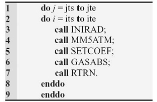
FIGURE 5.4. Code structure of RRTM‒LW scheme.
TABLE 5.1. Three Different Decomposition Methods and Their Corresponding Data Parallelism s (#DP)
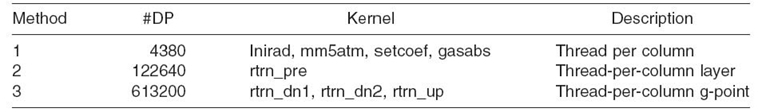
Each of these subroutines is implemented with a separate kernel except the last two ones that are too large to run efficiently as single kernels. GASABS is split into 16 kernels corresponding to the 16 longwave spectral bands, and RTRN is divided into 6 kernels. For most kernels, we assign each CUDA thread the workload of one “column.” In order to further exploit the fine-grained data parallelism, we even divide the workload of some kernels based on the layer or g-point dimension. Therefore, three decomposition strategies exist in our GPU implementation of RRTM‒LW and they result in three different data parallelisms as listed in Table 5.1.
Let Nx and Ny denote the latitudinal and longitudinal grid dimensions, respectively. The computations for the Nx × Ny “columns” are independent from each other, and we distribute the workload between CPUs and GPUs with the scheme presented in Section 5.3.3. The RRTM‒LW belongs to the EP problems and the skeleton of its MOC version is similar to Aigorithm 5.1. Hence, the detailed algorithm for MOC-RRTM is not shown here.
5.5 EXPERIMENTAL RESULTS
In this section, we first validate the workload distribution scheme with RRTM_LW, then perform NPB and RRTM‒LW on the TH-1A supercomputer and analyze their strong scalabilities.
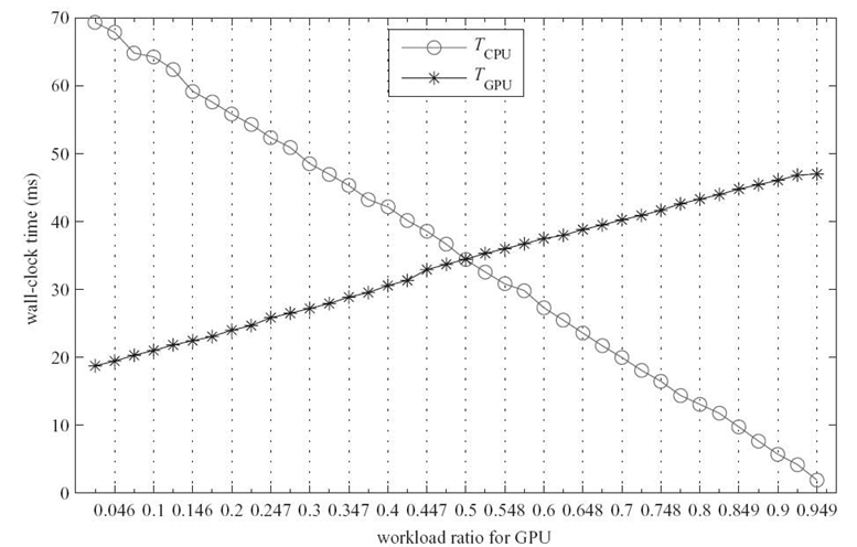
FIGURE 5.5. Results for RRTM‒LW with 73 × 60 horizontal grid points and 27 vertical levels. TCPU and TGPU is the wall-clock time for performing the workload assigned to CPUs and GPUs, respectively.
5.5.1 Validation of Workload Distribution Scheme
There are 12 CPU cores in each compute node of TH-1A supercomputer; hence, 12 OpenMP threads are spawned by each MPI process and Mn in Equation (5.3) is equal to 12. The workload of RRTM‒LW is distributed to CPU and GPU by splitting both the i and j loops depicted in Figure 5.4. We gradually decrease the GPU workload by 10 × PT ij-loops, where PT (i.e., 11 for TH-1A) denotes the number of OpenMP threads performing arithmetic operations in each compute node.
Figure 5.5 presents the results for RRTM‒LW (medium workload) with 73 × 60 horizontal grid points and 27 vertical levels. The predicted workload distribution ratio α relevant to the medium workload is 0.597 obtained by substituting S in Equation 5.3 with 16.3. However, Figure 5.5 shows that RRTM‒LW performs best when α reaches 0.5. We owe the deviation of 0.097 in workload distribution ratio to the start overhead TO of CUDA runtime environments. When only 4.6% workload is assigned to GPU, TGPU is still about 20 ms, most of which is contributed by TO. Consequently, TGPU is not proportional to workload distribution ratio α, which is different from TCPU.
To further validate our workload distribution scheme, we scale the workload downward and upward and present the results in Figure 5.6 (small workload) and Figure 5.7 (large workload), respectively. For RRTM‒LW with small workload, the relevant S is 10.37 and hence the predicted α is 0.485. Figure 5.6 portrays that TCPU equals TGPU when α reaches 0.376, which results in a deviation of 0.109 in the workload distribution ratio α. Similarly, the predicted α for RRTM‒LW with large workload is 0.601 obtained with the speedup S of 16.58. Note that RRTM‒LW achieves its best performance when α is about 0.532, and a deviation of 0.068 can also be observed.
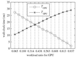
FIGURE 5.6. Results for RRTM‒LW with 42 × 42 horizontal grid points and 27 vertical levels.
FIGURE 5.7. Results for RRTM‒LW with 84 × 84 horizontal grid points and 27 vertical levels.
We observe that the actual workload distribution ratio α is always smaller than the predicated one for various workloads because of TO. In practical run, we can calculate the workload distribution ratio α based on Equation 5.3 and then amend it with an empirical value corresponding to TO of different workload scales.
5.5.2 Strong Scalability of EP and CG
There are many EP applications in the HPC community, such as Monte Carlo simulations, dense linear algebra applications (like DGEMM). EP is representative of applications in this category, and its relevant performance under different programming paradigms is portrayed in Figure 5.8. Note that the y-axis is in log scale and the execution configuration m × n denotes m compute nodes, each of which is launched with n MPI processes.
We observe that EP‒MPI achieves a speedup of 7.96 × at execution configuration 2048 × 1 over at 256 × 1, which demonstrates that EP‒MPI has a good strong scalability. For the EP‒MOC implementation, a maximal speedup of 55.8× is obtained at the execution configuration 256 × 1. When the number of MPI processes reach up to 2048, the performance speedup decreases to 33.7×, which mainly owes to the reduced workload for each MPI process.
Although GPUs are adept in dealing with computation-intensive applications, Figure 5.9 illustrates that memory-bounded applications like CG benchmark can still achieve great performance improvement through GPU acceleration. Compared with the CG‒MPI implementation, the CG‒MOC counterpart gains about 3.3 × performance at the execution configuration 64 × 1. When the number of compute nodes gradually increases up to 1024, the speedup decreases to 1.06, which is attributed to the relatively large overhead of data transferring between host and device memory against the decreasing workload for each GPU device.
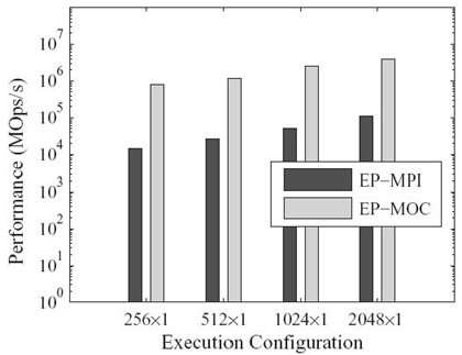
FIGURE 5.8. Performance comparison between MPI and MOC implementations of EP at class E.
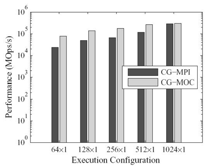
FIGURE 5.9. Performance comparison between MPI and MOC implementations of CG at class D.
It can be noticed that the 2× or 3× speedup is relatively small compared with that of the EP implementations. The reasons for this are as follows: (1) We maintain the CSR format of CG benchmark to storage the sparse matrix, which is not the best choice for the GPU hardware; (2) the launched threads are underutilized in our implementation. We utilize one 32-thread warp to compute the elements within each matrix row. However, the matrices in all the available workload scales of CG have fewer than 32 nonzero elements per row. For example, matrices in class D have 21 nonzero elements and in class E 26 nonzero entries. The matrix FEM/accelerator used in literature [26] has an average of 21.6 nonzero elements per row and a performance speedup of 2× is reported, which is analogous to our results.
5.5.3 Strong Scalability of RRTM‒LW
We integrate RRTM‒MOC implementation of RRTM‒LW into the WRF parallel benchmark (WPB) [29] and perform WPB on the 2.5-km case with up to 1024 compute nodes. The default WRF configuration is used. All the 12 CPU cores of each compute node are utilized: (1) 12 MPI processes are launched on these CPU cores for RRTM‒MPI, and (2) only 1 MPI process is launched on each compute node for RRTM‒MOC and 12 OpenMP threads are spawned by the MPI process. Figure 5.10 presents the wall-clock times for RRTM‒MPI and RRTM‒MOC on various processor scales.
It is observed that the wall-clock times for both RRTM‒MPI and RRTM‒MOC implementations drop linearly when the processor scale is gradually increased. Besides, the speedup fluctuates about 2.1 when the number of compute nodes increases from 256 to 1024, which demonstrates a good strong scalability. Note that the speedup decreases from 2.375 at 256 compute nodes to 2.077 at 1024 ones. We owe this to the shrinking computational workload for the relatively powerful GPUs.
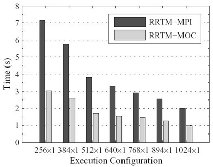
FIGURE 5.10. Performance comparison between MPI and MOC implementations of RRTM‒LW.
5.6 CONCLUSIONS
Scalability is a key concept for parallel computing on large-scale distributed systems. Many scalability metrics and models have been proposed for homogeneous and heterogeneous systems with traditional CPUs. However, the scalability for newly acknowledged heterogeneous CPU/GPU systems has not been well addressed. In this chapter, we have constructed a scalable hybrid programming pattern for large GPU clusters. Based on the TH-1A supercomputer, we have performed extensive experiments with several benchmarks and production codes to find the factors affecting the scalability for large-scale scientific and engineering applications. Experimental results show that the scalability of GPU applications is jointly determined by several factors, such as starting overhead of GPU computing environments, data-transfer cost between the host and the device memories, load imbalance, and MPI communication cost.
Although some factors for scalability of GPU applications have been identified, we have not reduced a comprehensive function on these factors, based on which we can further conduct a quantitative analysis. In the future, we will research more applications on GPU clusters and endeavor to obtain such scalability function after doing more experiments.
ACKNOWLEDGMENTS
This work was partially supported by the National Nature Science Foundation of China under Grant Nos. 60903042, 60736013, and 60872152, and by National 863 Plans Projects under Grant No.863-2010AA012404.
REFERENCES
[1] X.J. Yang, X.K. Liao, K. Lu, Q.F. Hu, J.Q. Song, and J.S. Su, “The TianHe-1A supercomputer: Its hardware and software,” Journal of Computer Science and Technology, 26(3): 344‒351, 2011.
[2] N.H. Sun, J. Xing, Z.G. Huo, G.M. Tan, J. Xiong, B. Li, and C. Ma, “Dawning Nebulae: A petaFLOPS supercomputer with a heterogeneous structure,” Journal of Computer Science and Technology, 26 (3): 352‒362, 2011.
[3] P. Jetley, L. Wesolowski, F. Gioachin, L.V. Kale, and T.R. Quinn, “Scaling hierarchical N-body simulations on GPU clusters,” in Proceedings of the 2010 ACM/IEEE Conference on Supercomputing, New Orleans, LA, pp. 1‒11, IEEE, 2010.
[4] T. Shimokawabe, T. Aoki, C. Muroi, J. Ishida, K. Kawano, T. Endo, A. Nukada, N. Maruyama, and K. Matsuoka, “An 80-fold speedup, 15.0 TFlops full GPU acceleration of non-hydrostatic weather model ASUCA production code,” in Proceedings of the 2010 ACM/IEEE Conference on Supercomputing, New Orleans, LA, pp. 1‒11, IEEE, 2010.
[5] D. Macri, “The scalability problem,” ACM Queue, 10(1): 66‒73, 2004.
[6] Y. Cui, K.B. Olsen, T.H. Jordan, K. Lee, J. Zhou, P. Small, D. Roten, G. Ely, D.K. Panda, A. Chourasia, J. Levesque, S.M. Day, and P. Maechling, “Scalable earthquake simulations on petascale supercomputers,” in Proceedings of the 2010 ACM/IEEE Conference on Supercomputing, New Orleans, LA, pp. 1‒20, IEEE, 2010.
[7] X.H. Sun, “Scalability versus execution time in scalable systems,” Journal of Parallel and Distributed Computing, 62: 173‒192, 2002.
[8] D. Muller-Wichards and W. Ronsch, “Scalability of algorithms: An analytic approach,” Parallel Computing, 21: 937‒952, 1995.
[9] P. Jogalekar and M. Woodside, “Evaluating the scalability of distributed systems,” IEEE Transactions on Parallel and Distributed Systems, 11(6): 589‒603, 2000.
[10] D. Goddeke, R. Strzodka, J. Mohd-Yusof, P. McCormick, S.H.M. Buijssen, M. Grajewski, and S. Turek, “Exploring weak scalability for FEM calculations on a GPU-enhanced cluster,” Parallel Computing, 33: 685‒699, 2007.
[11] H. Ltaief, S. Tomov, R. Nath, P. Du and J. Dongarra, “A scalable high performant Cholesky factorization for multicore with GPU accelerators,” in High Performance Computing for Computational Science-VECPAR 2010, pp. 93‒101, Springer-Verlag, 2010.
[12] I. Lashuk, A. Chandramowlishwaran, H. Langston, T.-A. Nguyen, R. Sampath, A. Shringarpure, R. Vuduc, L. Ying, D. Zorin, and G. Biros, “A massively parallel adaptive fast-multipole method on heterogeneous architectures,” in Proceedings of the 2009 ACM/IEEE Conference on Supercomputing, Portland, OR, pp. 1‒12, IEEE, 2009.
[13] S.R.M. Barros, D. Dent, L. Isaksen, G. Robinson, G. Mozdzynski, and F. Wollenweber, “The IFS model: A parallel production weather code,” Parallel Computing, 21(10): 1621‒1638, 1995.
[14] J. Michalakes, J. Dudhia, D. Gill, T. Henderson, J. Klemp, W. Skamarock, and W. Wang, “The weather research and forecast model: Software architecture and performance,” in Proceedings of the 11th ECMWF Workshop on the Use of High Performance Computing In Meteorology, Reading, UK, pp. 156‒168, 2004.
[15] J.E. Stone, D. Gohara, and G.C. Shi, “OpenCL: A parallel programming standard for heterogeneous computing systems,” Computing in Science and Engineering, 12(3): 66‒73, 2010.
[16] J. Dean and S. Ghemawat, “MapReduce: Simplified data processing on large clusters,” Communications of the ACM, 51(1): 107‒113, 2008.
[17] NPB homepage. Available at http://www.nas.nasa.gov/Resources/Software/npb.html. Accessed May 15, 2011.
[18] 36th TOP500 list. Available at http://www.top500.org/lists/2010/11. Accessed May 15, 2011.
[19] X.J. Yang, X.K. Liao, W.X. Xu, J.Q. Song, Q.F. Hu, J.S. Su, L.Q. Xiao, K. Lu, Q. Dou, J.P. Jiang, and C.Q. Yang, “TH-1: China's first petaflop supercomputer,”Frontiers of Computer science in china, 4(4): 445, 2010.
[20] MPI homepage. Available at http://www.mpi-forum.org∕. Accessed May 15, 2011.
[21] OpenMP homepage. Available at http://openmp.org∕wp∕. Accessed May 15, 2011.
[22] J. Nickolls, I. Buck, M. Garland, and K. Skadron, “Scalable parallel programming with CUDA,” ACM Queue, 6(2): 40‒53, 2008.
[23] K. Spafford, J. Meredith, J. Vetter, J. Chen, R. Grout, and R. Sankaran, “Accelerating S3D: A GPGPU case study,” in Euro-Par 2009 Workshops, LNCS 6043 (H.X. Lin, et al., eds.), pp. 122‒131, 2009.
[24] S.J. Park, J.A. Ross, D.R. Shires, D.A. Richie, B.J. Henz, and L.H. Nguyen, “Hybrid core acceleration of UWB SIRE radar signal processing,” IEEE Transactions on Parallel and Distributed Systems, 22(1): 46‒57, 2011.
[25] T. Yoshinaga and T.Q. Viet, “Optimization for hybrid MPI-OpenMP programs on a cluster of SMP PCs,” in Proceedings of Joint Japan-Tunisia Workshop on Computer Systems and Information Technology, Tokyo, Japan, pp. 1‒8, 2004.
[26] N. Bell and M. Garland, “Efficient sparse matrix-vector multiplication on CUDA,” Technical Report NVR-2008-004, NVIDIA Corporation, 2008.
[27] M.J. Iacono, E.J. Mlawer, S.A. Clough, and J.-J. Morcrette, “Impact of an improved long-wave radiation model, RRTM, on the energy budget and thermodynamic properties of the NCAR community climate mode, CCM3,” Journal of Geophysical Research, 105: 14873‒14890, 2000.
[28] J. Michalakes and M. Vachharajani, “GPU acceleration of numerical weather prediction,” Parallel Processing Letters, 18 (4): 531‒548, 2008.
[29] WPB homepage. Available at http: ∕∕www.mmm.ucar.edu∕WG2bench∕. Accessed May 15, 2011.