10

–––––––––––––––––––––––

Cost Optimization for Scalable Communication in Wireless Networks with Movement-Based Location Management

Keqin Li

10.1   INTRODUCTION

To effectively and efficiently deliver network services to mobile users in a wireless communication network, a key component of the network, that is, a dynamic location management scheme, should be carefully designed, and its cost should be thoroughly analyzed. There are two essential tasks in location management, namely, location update (location registration) and terminal paging (call delivery). Location update is the process for a mobile terminal to periodically notify its current location to a network so that the network can revise the mobile terminal's location profile in a location database. Terminal paging is the process for a network to search a mobile terminal by sending polling signals based on the information of its last reported location so that an incoming phone call can be routed to the mobile terminal.

Both location update and terminal paging consume significant communication bandwidth of a wireless network, battery power of mobile terminals, memory space in location registers and databases, and computing time at base stations. Therefore, both location update cost and terminal paging cost should be minimized. However, there is a trade-off between the cost of location update and the cost of terminal paging. More location updates reduce the cost of terminal paging, while insufficient location update increases the cost of terminal paging. A dynamic location management scheme has the capability to adjust its location update and terminal paging strategies based on the mobility pattern and incoming call characteristics of a mobile terminal, such that the combined cost of location update and terminal paging is minimized.

Analysis and minimization of the total location management cost for a single mobile terminal has been studied extensively by many researchers. However, there are two problems in existing research. First, cost of location update (measured by the number of location updates and related to resource consumption in base stations) and cost of terminal paging (measured by the number of cells in a paging area (PA) and related to communication bandwidth) are different in nature and difficult to be unified. Second, cost minimization should be carried out at the network level for multiple heterogeneous mobile terminals which simultaneously exist in a network and share network resources, not just for a single mobile terminal, so that network-wide performance optimization and network scalability can be considered. Hence, the traditional way of finding the best movement threshold that minimizes the total location management cost for a single mobile terminal might not be interesting and might not make much sense.

In this chapter, we consider the problem of cost optimization in wireless communication networks with movement-based location management. Our approach is to minimize the total cost of terminal paging of all mobile terminals with a constraint on the total cost of location update of all mobile terminals and to minimize the total cost of location update with a constraint on the total cost of terminal paging. These problems are formulated as multivariable optimization problems and are solved numerically. This approach allows network administration to freely control one of the total cost of location update and the total cost of terminal paging of all mobile terminals in a wireless network and to minimize the other. (This is not the case for a single mobile terminal, for which the determination of one cost also determines the other.) This is an effective way to handle cost trade-off, as in many other computing and communication systems. Such network-wide cost control and optimization is extremely important for scalable communication in a wireless network when the number of mobile terminals increases. Our approach also eliminates the issue of cost unification of location update and terminal paging since the two kinds of cost are separated. To the best of our knowledge, such cost optimization in an entire wireless communication network with heterogeneous mobile terminals has not been considered before.

The rest of the chapter is organized as follows. In Section 10.2, we provide necessary background information on dynamic location management in wireless communication networks. In Section 10.3, we discuss cost measure and optimization for a single mobile terminal. In Section 10.4, we define and solve the terminal paging cost minimization problem subject to constraint on location update cost. In Section 10.5, we define and solve the location update cost minimization problem subject to constraint on terminal paging cost. In Section 10.6, we present a numerical example. In Section 10.7, we summarize the chapter.

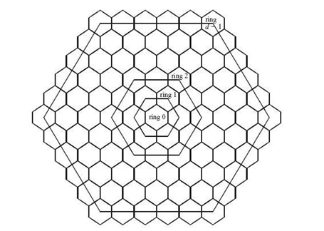
FIGURE 10.1. The hexagonal cell configuration.

10.2   BACKGROUND INFORMATION

Our model of a wireless communication network follows that in References 1. A wireless communication network has the common hexagonal cell configuration or mesh cell configuration. In the hexagonal cell structure (see Fig. 10.1), cells are hexagons of identical size and each cell has six neighbors. In the mesh cell structure (see Fig. 10.2), cells are squares of identical size and each cell has eight neighbors. Throughout the chapter, we let q be a constant such that q = 3 for the hexagonal cell configuration and q = 4 for the mesh cell configuration. By using the constant q, the hexagonal cell configuration and the mesh cell configuration can be treated in a unified way. For instance, we can say that each cell has 2q neighbors without mentioning the particular cell structure. The network is homogeneous in the sense that the behavior of a mobile terminal is statistically the same in all the cells.

Let s be the cell registered by a mobile terminal in the last location update. The cells in a wireless network can be divided into rings, where s is the center of the network and is called ring 0. The 2q neighbors of s constitute ring 1. In general, the neighbors of all the cells in ring r, except those neighbors in rings r‒ 1 and r, constitute ring r + 1. For all r ≥ 0, the cells in ring r have distance r to s. For all r ≥ 1, the number of cells in ring r is 2qr. Notice that the rings are defined with respect to s. When a mobile terminal updates its location to another cell s′, s′ becomes the center of the network, and ring r consists of the 2qr cells whose distance to s′ is r.

A mobile terminal u constantly moves from cell to cell. Such movement also results in movement from ring to ring. Let the sequence of cells visited by u before the next phone call be denoted as s₀, s₁, s₂,…, s_d,…, where s₀ = s is u’s last registered cell (not the cell in which u received the previous phone call) and considered as u’s current location. There are three location update methods proposed in the current literature, namely, the distance-based method, the movement-based method, and the time-based method.

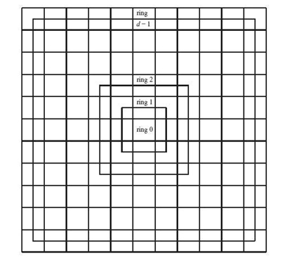
FIGURE 10.2. The mesh cell confi guration.

• In the distance-based location update method, location update is performed as soon as u moves into a cell s_j in ring d, where d is a distance threshold; that is, the distance of u from the last registered cell s is d, such that s_j is registered as u’s current location. It is clear that j ≥ d, that is, it takes at least d steps for u to reach ring d.
• In the movement-based location update method, location update is performed as soon as u has crossed cell boundaries for d times since the last location update, where d is a movement threshold. It is clear that the sequence of registered cells for u is s_d, s_2d, s_3d,….
• In the time-based location update method, location update is performed every τ units of time, where τ is a time threshold, regardless of the current location of u.

In all dynamic location management schemes, a current PA consists of rings 0, 1, 2,…, d − 1, where d is some value appropriately chosen. We say that such a PA has radius d. Since the number of cells in ring r is 2qr, for all r ≥ 1, the total number of cells in a PA is qd² − qd + 1. It should be noticed that a PA is defined with respect to the current location of a mobile terminal and is changed whenever a mobile terminal updates its location. The radius d of a PA can be adjusted in accordance with various cost and performance considerations. On the other hand, the location and size of a cell are fixed in a wireless network.

  We will consider two different call handling models:

• In the call plus location update (CPLU) model, the location of a mobile terminal is updated each time a phone call arrives; that is, in addition to distance-based or movement-based or time-based location updates, the arrival of a phone call also initiates location update and defines a new PA. This causes the original location update cycle of a mobile terminal being interrupted.
• In the call without location update (CWLU) model, the arrival of a phone call has nothing to do with location update; that is, a mobile terminal still keeps its original location update cycles.

Our cost analysis and optimization will be conducted for both models.

For a random variable T, we use E(T) to represent the expectation of T and λT = E(T)⁻¹. The probability density function (pdf) of T is f_T(t). There are two important random variables in the study of dynamic location management. The intercall time T_c is defined as the length of the time interval between two consecutive phone calls. The cell residence time T_s is defined as the time a mobile terminal stays in a cell before it moves into a neighboring cell. The quantity ρ = λ_Tc/λ_Ts is the call-to-mobility ratio.

The cost of dynamic location management contains two components, that is, the cost of location update and the cost of terminal paging. The cost of location update is proportional to the number of location updates. If there are X_u location updates between two consecutive phone calls, the cost of location update is Δ_uX_u, where Δ_u is a constant. Since X_u is a random variable, the location update cost is actually calculated as Δ_u(EX_u). The cost of terminal paging is proportional to the number of cells paged. If a PA has radius d, the cost of paging is Δ_p(qd² − qd + 1), where Δ_p is a constant.

Dynamic location management is per-terminal based. A mobile terminal is specified by f_Tc(t) and f_Ts(t), where f_Tc (t) is the call pattern and f_Ts (t) is the mobility pattern. Since a location update method determines the location update cost and a terminal paging method determines the terminal paging cost, for given a mobile terminal, we need to find a balanced combination of a location update method and a terminal paging method, such that the total location management cost for the mobile terminal is minimized.

Dynamic location management has been studied extensively by many researchers. The performance of movement-based location management schemes has been investigated in References 2‒9. The performance of distance-based location management schemes has been studied in References 3 and 10‒14. The performance of time-based location management schemes has been considered in References 3 and 15‒17. Terminal paging methods with low cost and time delay have been studied by several researchers [2, 12, 18‒22]. Others studied were reported in References 23‒ 32. Dynamic location management in a wireless communication network with a finite number of cells has been treated as an optimization problem that is solved by using bioinspired methods such as simulated annealing, neural networks, and genetic algorithms [33‒ 38]. The reader is also referred to the surveys in References 39‒ 42 (Chapter 15) and 43 Chapter 11.

10.3   COST MEASURE AND OPTIMIZATION FOR A SINGLE USER

Minimization of total location management cost for a single mobile terminal has been studied extensively. Traditionally, the performance measure for a single mobile user is the cost of location management (including the cost of location update and the cost of terminal paging) between two consecutive phone calls. However, different mobile terminals have different intercall times. Our performance measure in this chapter is the cost of location management per unit of time so that the cost of different users can be added.

In this chapter, we will focus on the movement-based location update method. Our investigation in this chapter is based on our recent work in References 1, where we successfully developed closed-form expressions of location update cost for a mobile terminal under both CPLU and CWLU models.

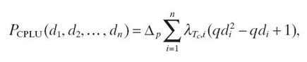
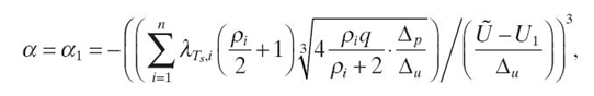
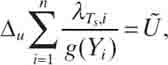
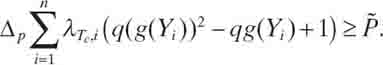
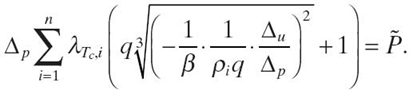
The following theorem gives the cost of location management per unit of time for a single mobile user under the CPLU model. Theorem 10.1   If   f_Ts(t) has an Erlang distribution, the total cost of location management per unit of time under the CPLU model is

where ρ = λ_Tc/λ_Ts, for any probability distribution f_Tc(t).

Proof: It was proven in Reference 1 that if f_Ts(t) has an Erlang distribution, the total cost of location management between two consecutive phone calls under the CPLU model is

for any probability distribution f_Ts(t). Since there are λ_Tc phone calls per unit of time, we get the theorem.     ■

The following theorem gives the cost of location management per unit of time for a single mobile user under the CWLU model.

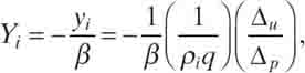
Theorem 10.2    The total cost of location management per unit of time under the CWLU model is

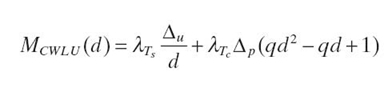
for any probability distributions f_Ts(t) and f_Ts(t).

Proof: It was proven in Reference 1 that for any probability distributions f_Ts(t) and f_Ts(t) the total cost of location management between two consecutive phone calls under the CWLU model is

Since there are λ_Tc phone calls per unit of time, we get the theorem.      ■

Let us consider the derivative of M_CPLU(d) in Theorem 10.1 for the CPLU model:

that is,

which yields

where

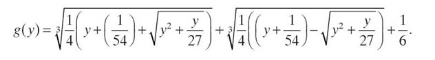
It can be verified that 2d³−d² ≥ 0 if d ≥ 1/2, and 2d³ − d² is an increasing function in the range [1/2, ∞). Thus, for y ≥ 0, there is a unique solution: d ∈ [1/2, ∞), which satisfies 2d³−d² = y. Furthermore, d ≥ 1 if and only if y ≥ 1. To ensure that there is a solution of d ≥ 1, we assume that y_CPLU ≥ 1. The above equation of d can be solved using basic algebra, and the solution is given below. We define a function g(y) as

We have the following theorem.

Theorem 10.3    The optimal value of the movement threshold which minimizes M_CPLU(d) is either ⌊d⌋ or ⌈d⌉, where d = g(y_CPLU), whichever minimizes M_CPLU(d).

Let us consider the derivative of M_CWLU(d) in Theorem 10.2 for the CWLU model:

that is,

which yields

where

Again, we assume that y_CWLU ≥ 1. The above equation of d can be solved using basic algebra, and the solution is given below.

Theorem 10.4    The optimal value of the movement threshold which minimizes M_CWLU(d) is either ⌊d⌋ or ⌈d⌉, where where d = g(y_CWLU), whichever minimizes M_CWLU(d).

10.4   COST OPTIMIZATION WITH LOCATION UPDATE CONSTRAINT

In this section, we consider the terminal paging cost minimization problem with constraint on location update cost.

10.4.1   The CPLU Model

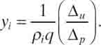
Assume that there are n heterogeneous mobile terminals u₁, u₂,…, u_n in a wireless communication network. Each u_i has λ_{Tc, i}, λ_{Ts, i}, ρ_i = λ_{Tc, i}, /λ_{Ts, i} and

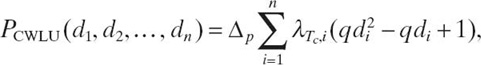
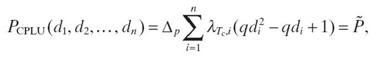
where 1≤ i ≤ n. We are going to minimize the total cost of terminal paging of all mobile terminals per unit of time, which is defined as a function of d₁, d₂,…, d_n; that is,

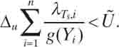
with a constraint on the total cost of location update of all mobile terminals per unit of time; that is,

where

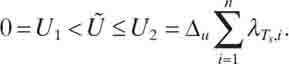
Notice that the lower bound U₁ for Ũ is the total cost of location update of the n mobile terminals per unit of time when all the d_i's are infinity. The upper bound U₂ for Ũ is the total cost of location update of the n mobile terminals per unit of time when all the d_i's are 1. For mathematical convenience, we treat the d_i's as continuous variables in the range [1/2, ∞).

To minimize P_CPLU(d₁, d₂,…, d_n), we establish a Lagrange multiplier system:

where α is a Lagrange multiplier. The above equation implies that

that is,

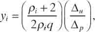
for all 1 ≤ i ≤ n. From the last equation, we get

where

which implies that

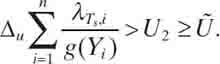
Substituting d₁, d₂,…, d_n into the constraint

we obtain

What remains to be done is to solve the above equation of α.

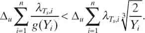
It is easy to see that the left-hand side of the last equation is an increasing function of α in the range (−∞, 0]. To find α, we need to find α₁ and α₂, such that α is guaranteed in the range [α₁, α₂]. We notice that

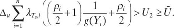
Therefore, we have

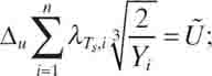
We further let

that is,

or

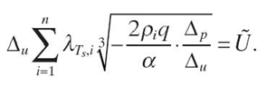
The last equation implies that if

we have

We also notice that g(0) = 1/2 < 1. Hence, if α = α₂ = 0, we have

The classical bisection method can be employed to search for a numerical solution to α in the range [α₁, α₂].

10.4.2   The CWLU Model

The terminal paging cost minimization problem with constraint on location update cost for the CWLU model is described and solved in a way similar to that for the CPLU model. Each u_i has λ_{Tc, i}, λ_{Ts, i} and ρ_i = λ_{Tc, i}, / λ_{Ts, i}. Let

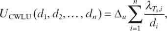
We are going to optimize the total cost of terminal paging of all mobile terminals per unit of time; that is,

subject to the constraint

where

Notice that the lower bound U₁ is the total cost of location update of the n mobile terminals per unit of time when all the d_i's are infinity. The upper bound U₂ is the total cost of location update of the n mobile terminals per unit of time when all the d_i's are 1.

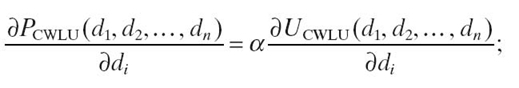
To minimize P_CWLU (d₁, d₂,…, d_n), we establish a Lagrange multiplier system,

where λ is a Lagrange multiplier. The above equation implies that

that is,

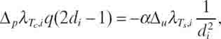
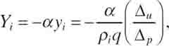
for all 1 ≤ i ≤ n. From the last equation, we get

where

which implies that

Substituting d₁, d₂,…, d_n into the constraint

we obtain

which gives an equation of α.

To solve the above equation of α, we need to find α₁ and α₂, such that α is guaranteed in the range [α₁, α₂]. By using the fact that we obtain

Let

that is,

The last equation implies that if

we have

It is clear that if α = α₂ = 0, we have

Again, we can use the classical bisection method to search for a numerical solution to α in the range [α₁, α₂].

10.5   COST OPTIMIZATION WITH TERMINAL PAGING CONSTRAINT

We now consider the location update cost minimization problem with constraint on terminal paging cost.

10.5.1   The CPLU Model

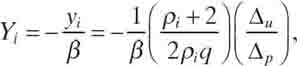
Assume that there are n heterogeneous mobile terminals u₁, u₂,…, u_n in a wireless communication network. Each u_i has λ_{Tc, i}, λ_{Ts, i}, ρ_i = λ_{Tc, i}, /λ_{Ts, i} and

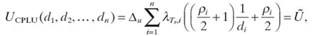
here 1 ≤ i ≤ n. We are going to minimize the total cost of location update of all mobile terminals per unit of time, which is defined as a function of d₁, d₂,…, d_n; that is,

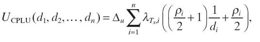
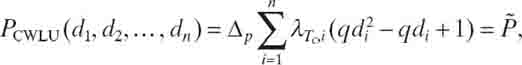
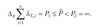
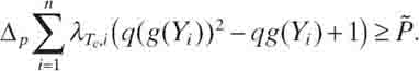
with a constraint on the total cost of terminal paging of all mobile terminals per unit of time; that is,

where

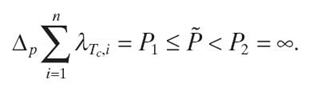
Notice that the lower bound P₁ for P~ is the total cost of terminal paging of the n mobile terminals per unit of time when all the d_i's are 1. The upper bound P₂ for P~ is the total cost of terminal paging of the n mobile terminals per unit of time when all the d_i's are infinity.

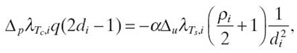
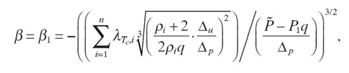
To minimize U_CPLU(d₁, d₂,…, d_n), we establish a Lagrange multiplier system:

where β is a Lagrange multiplier. The above equation implies that

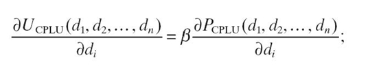
that is,

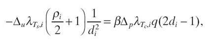
for all 1 ≤ i ≤ n. From the last equation, we get

where

which implies that

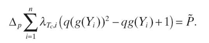
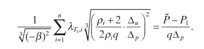
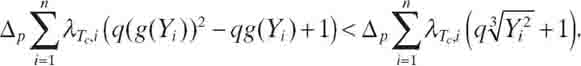
Substituting d₁, d₂,…, d_n into the constraint

we obtain

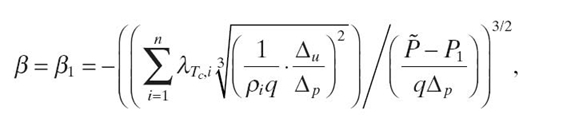
What remains to be done is to solve the above equation of β.

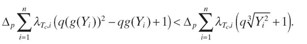
It is easy to see that the left-hand side of the last equation is an increasing function of β in the range (‒∞, 0). To find β, we need to find β₁ and β₂, such that β is guaranteed in the range [ β₁, β₂]. We notice that

if y ≥ 1. Therefore, we have

We further let

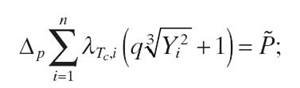
that is,

or

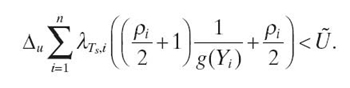
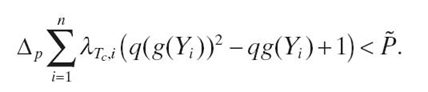
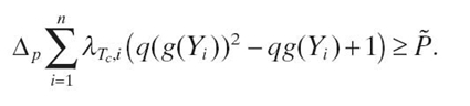
The last equation implies that if

we have

As for β₂, we need to choose β₂, which is sufficiently close to 0, such that

Thus, we must have β ∈ [β₁, β₂], which can be found by using the bisection method.

10.5.2   The CWLU Model

The location update cost minimization problem with constraint on terminal paging cost for the CWLU model is formulated and solved in a way similar to that for the CPLU model. Each u_i has λ_{Tc, i}, λ_{Ts, i} and ρ_i = λ_{Tc, i}/λ_{Ts, i}. Let

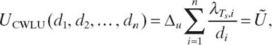
We are going to optimize the total cost of location update of all mobile terminals per unit of time; that is,

subject to the constraint

where

Notice that the lower bound P₁ is the total cost of terminal paging of the n mobile terminals per unit of time when all the d_i's are 1. The upper bound P₂ is the total cost of terminal paging of the n mobile terminals per unit of time when all the d_i's are infinity.

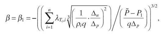
To minimize U_CWLU(d₁, d₂,…, d_n), we establish a Lagrange multiplier system:

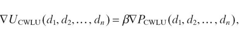
where β is a Lagrange multiplier. The above equation implies that

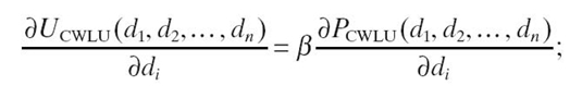
that is,

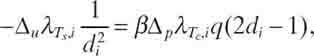
for all 1 ≤ i ≤ n. From the last equation, we get

where

which implies that

Substituting d₁, d₂,…, d_n into the constraint

we obtain

which gives an equation of β .

To solve the above equation of β, we need to find β₁ and β₂, such that β is guaranteed in the range [β₁, β₂]. By using the fact that , we obtain

Let

that is,

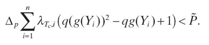
The last equation implies that if

we have

As for β₂, we need to choose β₂, which is sufficiently close to 0, such that

A numerical solution to β can be found by using the bisection method.

10.6   NUMERICAL DATA

In this section, we demonstrate numerical data.

 We consider n = 9m mobile terminals classified into nine categories:

• few calls with low mobility: λ_{Tc, i} = 1, λ_{Ts, i} = 10, ρ = 0.1.
• few calls with moderate mobility: λ_{Tc, i} = 1, λ_{Ts, i} = 30, ρ = 0.03.
• few calls with high mobility: λ_{Tc, i} = 1, λ_{Ts, i} = 100 ρ = 0.01.
• moderate calls with low mobility: λ_{Tc, i} = 5, λ_{Ts, i} = 10, ρ = 0.5.
• moderate calls with moderate mobility: λ_{Tc, i} = 5, λ_{Ts, i} = 30, ρ = 0.17.
• moderate calls with high mobility: λ_{Tc, i} = 5, λ_{Ts, i} = 100, ρ = 0.05.
• many calls with low mobility: λ_{Tc, i} = 20, λ_{Ts, i} = 10, ρ = 2.
• many calls with moderate mobility: λ_{Tc, i} = 20, λ_{Ts, i} = 30, ρ = 0.67.
• many calls with high mobility: λ_{Tc, i} = 20, λ_{Ts, i} = 100, ρ = 0.2.

The number of mobile terminals in each category is m = 10.

We set the parameters Δ_p and Δ_u as Δ_p = 1 and Δ_u = 10, 20, 30, 40.

In Figures 10.3‒ 10.6, we display the impact of location update constraint on terminal paging cost optimization for the CPLU model with q = 3 in Figure 10.3, the CWLU model with q = 3 in Figure 10.4, the CPLU model with q = 4 in Figure 10.5, and the CWLU model with q = 4 in Figure 10.6. Each curve shows the terminal paging cost P_CPLU(d₁, d₂,…, d _n) or P_CWLU (d₁, d₂,…, d_n) (divided by 10⁴) versus Ũ (divided by 10⁴). The interval [U₁, U₂] shifts to the right on the Ũ-axis and the length of the interval increases as Δ_u increases. It is observed that in the range [U₁ + (U₂ − U₁)/3, U₂], P_CPLU(d₁, d₂,…, d_n) or P_CWLU (d₁, d₂,…, d_n). increases smoothly as Ũ decreases. However, further reduction of Ũ, that is, more location update constraint, causes dramatic increase in P_CPLU(d₁, d₂,…, d_n) or P_CWLU(d₁, d₂,…, d_n) due to the quadratic terminal paging cost.

FIGURE 10.3. Optimization with location update constraint (CPLU, q = 3).

FIGURE 10.4. Optimization with location update constraint (CWLU, q = 3).

FIGURE 10.5. Optimization with location update constraint (CPLU, q = 4).

FIGURE 10.6. Optimization with location update constraint (CWLU, q = 4).

In Figures 10.7‒10.10, we display the impact of terminal paging constraint on location update cost optimization for the CPLU model with q = 3 in Figures 10.7, the CWLU model with q = 3 in Figures 10.8, the CPLU model with q = 4 in Figures 10.9, and the CWLU model with q = 4 in Figures 10.10. Each curve shows the location update cost U_CPLU(d₁, d₂,…, d_n) or U_CWLU(d₁, d₂,…, d_n) (divided by 10⁴) versus (divided by 10⁴). It is observed that as increases, U_CPLU(d₁, d₂,…, d_n) or U_CWLU(d₁, d₂,…, d_n) decreases smoothly.

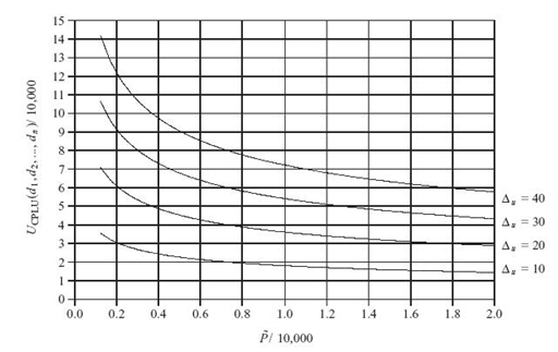
FIGURE 10.7. Optimization with terminal paging constraint (CPLU, q = 3).

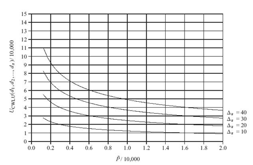
FIGURE 10.8. Optimization with terminal paging constraint (CWLU, q = 3).

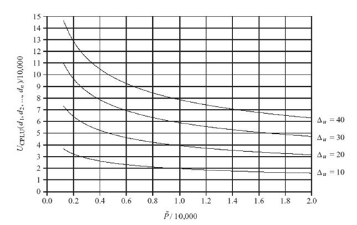
FIGURE 10.9. Optimization with terminal paging constraint (CPLU, q = 4).

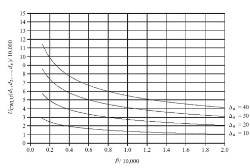
FIGURE 10.10. Optimization with terminal paging constraint (CWLU, q = 4).

10.7   CONCLUDING REMARKS

We have emphasized the motivation and significance of network-wide cost control and optimization for scalable communication in a wireless network with heterogeneous mobile terminals. Our approach is to minimize one of the total cost of location update and the total cost of terminal paging of all mobile terminals in a wireless network by fixing the other. Our cost minimization problems are formulated as multivariable optimization problems and are solved numerically for the CPLU model and the CWLU model. Our approach eliminates the issue of cost unification of location update and terminal paging since the two kinds of cost are separated. The model and method developed in this chapter provide an effective way to handle cost trade-off in large-scale wireless communication networks.

REFERENCES

[1] K. Li, “Cost analysis and minimization of movement-based location management schemes in wireless communication networks: A renewal process approach,” Wireless Networks, 17(4): 1031‒1053, 2011.

[2] I.F. Akyildiz, J.S.M. Ho, and Y.-B. Lin, “Movement-based location update and selective paging for PCS networks,” IEEE/ACM Transactions on Networking, 4: 629‒638, 1996.

[3] A. Bar-Noy, I. Kessler, and M. Sidi, “Mobile users: To update or not update?” Wireless Networks, 1: 175‒185, 1995.

[4] Y. Fang, “Movement-based mobility management and trade off analysis for wireless mobile networks,” IEEE Transactions on Computers, 52(6): 791‒803, 2003.

[5] J. Li, H. Kameda, and K. Li, “Optimal dynamic mobility management for PCS networks,” IEEE/ACM Transactions on Networking, 8(3): 319‒327, 2000.

[6] J. Li, Y. Pan, and X. Jia, “Analysis of dynamic location management for PCS networks,” IEEE Transactions on Vehicular Technology, 51(5): 1109‒1119, 2002.

[7] Y.-B. Lin, “Reducing location update cost in a PCS network,” IEEE/ACM Transactions on Networking, 5(1): 25‒33, 1997.

[8] R.M. Rodr í guez-Dagnino and H. Takagi, “Movement-based location management for general cell residence times in wireless networks,” IEEE Transactions on Vehicular Technology, 56(5): 2713‒2722, 2007.

[9] Y. Zhang, J. Zheng, L. Zhang, Y. Chen, and M. Ma, “Modeling location management in wireless networks with generally distributed parameters,” Computer Communications, 29(12): 2386‒2395, 2006.

[10] A. Abutaleb and V.O.K. Li, “Location update optimization in personal communication systems,” Wireless Networks, 3(3): 205‒216, 1997.

[11] V. Casares-Giner and J. Mataix-Oltra, “Global versus distance-based local mobility tracking strategies: A unified approach,” IEEE Transactions on Vehicular Technology, 51(3): 472‒485, 2002.

[12] J.S.M. Ho and I.F. Akyildiz, “Mobile user location update and paging under delay constraints,” Wireless Networks, 1: 413‒425, 1995.

[13] U. Madhow, M.L. Honig, and K. Steiglitz, “Optimization of wireless resources for personal communications mobility tracking,” IEEE/ACM Transactions on Networking, 3(12): 698‒707, 1995.

[14] C.K. Ng and H.W. Chan, “Enhanced distance-based location management of mobile communication systems using a cell coordinates approach,” IEEE Transactions on Mobile Computing, 4(1): 41‒55, 2005.

[15] I.F. Akyildiz and J.S.M. Ho, “Dynamic mobile user location update for wireless PCS networks,” Wireless Networks, 1: 187‒196, 1995.

[16] F.V. Baumann and I.G. Niemegeers, “An evaluation of location management procedures,” in Proceedings of IEEE International Conference on Universal Personal Communications, pp. 359‒364, 1994.

[17] C. Rose, “Minimizing the average cost of paging and registration: A timer-based method,” Wireless Networks, 2(2): 109‒116, 1996.

[18] A. Abutaleb and V.O.K. Li, “Paging strategy optimization in personal communication systems,” Wireless Networks, 3(3): 195‒204, 1997.

[19] A. Bar-Noy, Y. Feng, and M.J. Golin, “Paging mobile users efficiently and optimally,” in Proceedings of the 26th IEEE International Conference on Computer Communications, pp. 1910‒1918, 2007.

[20] C. Rose and R. Yates, “Minimizing the average cost of paging under delay constraints,” Wireless Networks, 1: 211‒219, 1995.

[21] M. Verkama, “Optimal paging—A search theory approach,” in Proceedings of IEEE International Conference on Universal Personal Communications, pp. 956‒960, 1996.

[22] W. Wang, I.F. Akyildiz, G.L. Stüber, and B.-Y. Chung, “Effective paging schemes with delay bounds as QoS constraints in wireless systems,” Wireless Networks, 7: 455‒466, 2001.

[23] I.F. Akyildiz and W. Wang, “A dynamic location management scheme for next-generation multitier PCS systems,” IEEE Transactions on Wireless Communications, 1(1): 178‒189, 2002.

[24] T.X. Brown and S. Mohan, “Mobility management for personal communications systems,” IEEE Transactions on Vehicular Technology, 46(2): 269‒278, 1997.

[25] E. Cayirci and I.F. Akyildiz, “User mobility pattern scheme for location update and paging in wireless systems,” IEEE Transactions on Mobile Computing, 1(3): 236‒247, 2002.

[26] P.G. Escalle, V.C. Giner, and J.M. Oltra, “Reducing location update and paging costs in a PCS network,” IEEE Transactions on Wireless Communications, 1(1): 200‒209, 2002.

[27] Y. Fang, “General modeling and performance analysis for location management in wireless mobile networks,” IEEE Transactions on Computers, 51(10): 1169‒1181, 2002.

[28] Y. Fang, I. Chlamtac, and Y.-B. Lin, “Potable movement modeling for PCS networks,” IEEE Transactions on Vehicular Technology, 49(4): 1356‒1363, 2000.

[29] C. Rose, “State-based paging/registration: A greedy technique,” IEEE Transactions onIEEE Vehicular Technology, 48(1): 166‒173, 1999.

[30] C.U. Saraydar, O.E. Kelly, and C. Rose, “One-dimensional location area design,” Transactions on Vehicular Technology, 49(5): 1626‒1632, 2000.

[31] G. Wan and E. Lin, “Cost reduction in location management using semi-realtime movement information,” Wireless Networks, 5: 245‒256, 1999.

[32] A. Yener and C. Rose, “Highly mobile users and paging: Optimal polling strategies,” IEEE Transactions on Vehicular Technology, 47(4): 1251‒1257, 1998.

[33] E. Alba, J. García-Nieto, J. Taheri, and A. Zomaya, “New research in nature inspired algorithms for mobility management in GSM networks,” Lecture Notes in Computer Science, 4974: 1‒10, 2008.

[34] R. Subratal and A.Y. Zomaya, “Dynamic location management for mobile computing,” Telecommunication Systems, 22(1‒4): 169‒187, 2003.

[35] J. Taheri and A.Y. Zomaya, “A simulated annealing approach for mobile location management,” Computer Communications, 30(4): 714‒730, 2007.

[36] J. Taheri and A.Y. Zomaya, “A combined genetic-neural algorithm for mobility management,” Journal of Mathematical Modelling and Algorithms, 6(3): 481‒507, 2007.

[37] J. Taheri and A.Y. Zomaya, “Clustering techniques for dynamic location management in mobile computing,” Journal of Parallel and Distributed Computing, 67(4): 430‒447, 2007.

[38] J. Taheri and A.Y. Zomaya, “Bio-inspired algorithms for mobility management,” in Proceedings of the International Symposium on Parallel Architectures, Algorithms, and Networks, pp. 216‒223, 2008.

[39] I.F. Akyildiz, J. McNair, J.S.M. Ho, H. Uzunalioğlu, and W. Wang, “Mobility management in next-generation wireless systems,” Proceedings of the IEEE, 87(8): 1347‒1384, 1999.

[40] N.E. Kruijt, D. Sparreboom, F.C. Schoute, and R. Prasad, “Location management strategies for cellular mobile networks,” IEE Electronics & Communication Engineering Journal, 10 (2): 64‒72, 1998.

[41] S. Tabbane, “Location management methods for third-generation mobile systems,” IEEE Communications Magazine, vol. 35, pp. 72‒84, 1997.

[42] B. Furht and M. Ilyas, eds., Wireless Internet Handbook—Technologies, Standards, and Applications. Boca Raton, FL: CRC Press, 2003.

[43] S.G. Glisic, Advanced Wireless Networks—4G Technologies. Chichester, England: John Wiley & Sons, 2006.