21

–––––––––––––––––––––––

Implementing Pointer Jumping for Exact Inference on Many-Core Systems

Yinglong Xia, Nam Ma, and Viktor K. Prasanna

21.1 INTRODUCTION

Many recent parallel computing platforms install many-core processors or multiple multicore processors to deliver high performance. Such platforms are known as many-core systems, for example, the 24-core AMD Magny-Cours system, 32-core Intel Nehalem-EX system, 64-hardware-thread UltraSPARC T2 (Niagara 2) Sun Fire T2000 [1], and 80-core IBM Cyclops64 [2]. To accelerate the execution of applications in a many-core system, we must keep the cores busy. However, as the number of cores increases, a fundamental challenge in parallel computing is how to keep many cores busy, especially for applications with inherently sequential computation.

Pointer jumping is a parallel computing technique for exploring parallel activities from applications [3]. In this chapter, we especially consider applications offering limited parallelism. Such applications typically consist of a few long chains in their structures, where the computation along a chain must be performed sequentially. However, we can leverage pointer jumping to find more parallelism so that we can keep more cores busy simultaneously and therefore improve the overall performance.

We use a sample application called exact inference in junction trees to discuss the implementation of pointer jumping in many-core systems [4]. A junction tree is a probabilistic graphical model that can be used to model many real-world systems [5]. Each node in a junction tree is called a clique, consisting of a set of random variables. Each edge represents the shared variables between two adjacent cliques. Inference is the computation of the conditional probability of a set of random variables, given knowledge of another set of random variables. Existing parallel techniques for exact inference explore data parallelism and structural parallelism [6]. However, if a junction tree consists of only a few long chains, it is not straightforward to find enough parallelism for keeping all the cores busy in a many-core system.

In this chapter, we have the following contributions: (1) We adapt the pointer jumping for exact inference in junction trees. The proposed method is suitable for junction trees offering limited data parallelism and structural parallelism. (2) We analyze the impact of the number of cores on the speedup of the proposed method with respect to a serial algorithm. (3) We implement the proposed method using Pthreads on two state-of-the-art many-core systems. (4) We evaluate our implementation and compare it with our baseline method exploiting structural parallelism.

The rest of the chapter is organized as follows: In Section 21.2, we review pointer jumping and exact inference in junction trees. Section 21.3 discusses related work. Sections 21.4 and 21.5 present our proposed algorithm and its performance analysis. Section 21.6 discusses how to generalize the proposed work. We describe our implementation and experiments in Section 21.7 and then conclude the chapter in Section 21.8.

21.2 BACKGROUND

21.2.1 Pointer Jumping

Pointer jumping is a parallel technique used in computations with inherently sequential operations, such as finding the prefix sum for a list of data [3, 7]. Given a list of N elements, pointer jumping allows data transfer from each node to all of its successors in log N iterations, whereas the serial transfer takes O(N) iterations. Figure 21.1 illustrates the iterations of pointer jumping on a list of N elements. Initially, only has the updated data. Let pa denote the parent of , that is, , 0 < i ≤ N − 1. We propagate the data from to the rest of the nodes as follows: In the first iteration, we transfer data from pa to for each i ∈ {1…N} in parallel. Then, for each node, we let the pointer to its parent jump to its grandparent, that is, letting pa² = pa(pa ). After log N iterations, all the elements complete transferring their data to their successors, as shown in Figure 21.1.

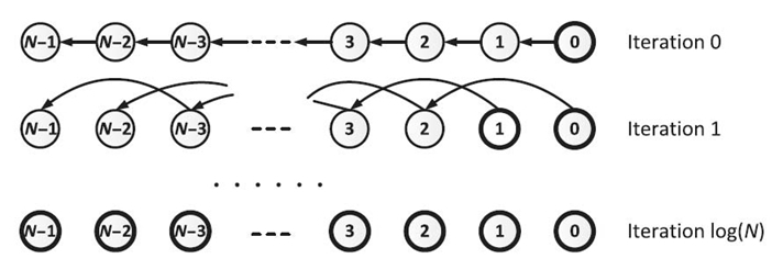
FIGURE 21.1. Pointer jumping on a list.

On the concurrent-read exclusive-write parallel random access machine (CREW-PRAM) [3] with P processors, 1 ≤ P ≤ N, each element of the list is assigned to a processor. Note that the update operations are implicitly synchronized at the end of each pointer jumping iteration. Each iteration takes O(N/P) time to complete O(N) update operations. Thus, the pointer jumping-based algorithm runs in O((N. logN)/P) time using a total number of O(N log N) update operations.

21.2.2 Exact Inference

A Bayesian network is a probabilistic graphical model that exploits conditional independence to compactly represent a joint distribution. Figure 21.2a shows a sample Bayesian network, where each node represents a random variable. Each edge indicates the probabilistic dependence between two random variables. The evidence in a Bayesian network is the set of instantiated variables. Exact inference in a Bayesian network is the computation of updating the conditional distribution of the random variables given the evidence.

Exact inference using Bayes'theorem fails for networks with undirected cycles [6]. Most methods convert a Bayesian network to a cycle-free hypergraph called a junction tree. We illustrate a junction tree converted from the Bayesian network in Figure 21.2 a. Each vertex in Figure 21.2 b is called a clique, which contains multiple random variables from the Bayesian network. We use the following notations in this chapter. A junction tree is represented as , where represents a tree and denotes the parameters in the tree. Given adjacent cliques and the separator is defined as is a set of potential tables. The potential table of denoted can be viewed as the joint distribution of the random variables in . For a clique with w variables, each having r states, the number of entries in is r^w [4].

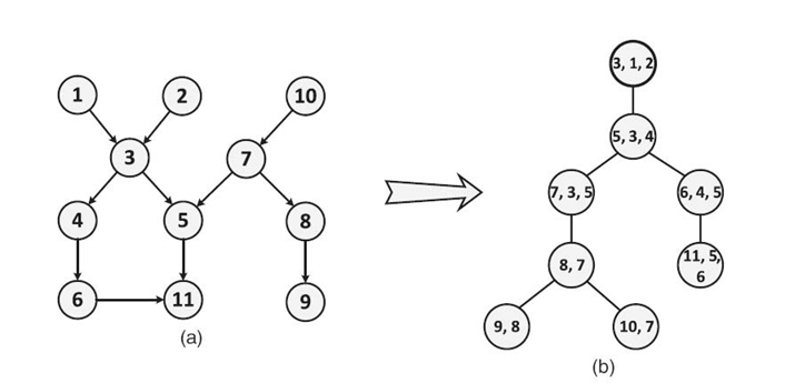
FIGURE 21.2. (a) A sample Bayesian network and (b) the corresponding junction tree.

In a junction tree, exact inference is performed as follows: Assuming evidence is E = {A_i = a} and A_i ∈ , E is absorbed at by instantiating the variable A_i and renormalizing the remaining variables of the clique. The evidence is then propagated from to any adjacent cliques Let denote the potential table of after E is absorbed, and the potential table of Mathematically, evidence propagation is represented as [6]

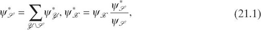
where is a separator between cliques and denotes the original(updated) potential table of is the updated potential table of A junction tree is updated using the above evidence propagation in two phases, that is, evidence collection and evidence distribution. In evidence collection, evidence is propagated from the leaves to the root. A clique is ready to propagate evidence to its parent when has already been updated, that is, when all of the children of have finished propagating evidence to . Evidence distribution is the same as collection, except that the evidence propagation direction is from the root to the leaves. The two phases ensure that evidence at any cliques can be propagated to all the other cliques [6].

21.3 RELATED WORK

There are several works on parallel exact inference. In Reference 8, the authors explore structural parallelism in exact inference by assigning independent cliques to separate processors for concurrent processing. In Reference 9, structural parallelism is explored by a dynamic task scheduling method, where the evidence propagation in each clique is viewed as a task. Unlike the above techniques, data parallelism in exact inference is explored in Reference 8, 10 and 11. Since these solutions partition potential tables and update each part in parallel, they are suitable for junction trees with large potential tables. If the input junction tree offers limited structural and data parallelism, the performance of the above solutions are adversely affected.

Pointer jumping has been used in many algorithms, such as list ranking, parallel prefix [3]. In Reference 12, the authors use pointer jumping to develop a new spanning tree algorithm for symmetric multiprocessors that achieves parallel speedups on arbitrary graphs. In Reference 5, the authors propose a pointer jumping-based method for exact inference in Bayesian networks. The method achieves logarithmic execution time regardless of structural or data parallelism in the networks. However, the method proposed in Reference 5 exhibits limited performance for multiple evidence inputs. In addition, no experimental study has been provided Reference 5. Our proposed algorithm combines the pointer jumping technique with Lauritzen and Spiegelhalter's two-phase algorithm, which is efficient for multiple evidence inputs.

21.4 POINTER JUMPING-BASED ALGORITHMS FOR SCHEDULING EXACT INFERENCE

21.4.1 Evidence Propagation in Chains

We formulate evidence propagation in a chain of N cliques as follows. Let clique = {S_{i + 1, i}, V_i, S_{i−1, i}}, where separator and . For the sake of simplicity, we let S_{0, − 1} = S_{N, N−1} = Ø and joint probability . We rewrite as a conditional distribution:

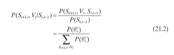
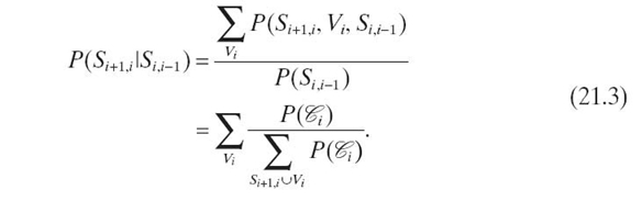
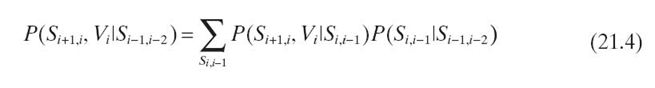
Using Equations (21.2) and (21.3), in iteration 0, we propagate the evidence from pa to by

In iteration k, we propagate evidence from pa^2k to by

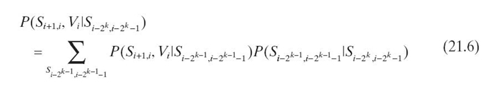
Performing Equations (21.6) and (21.7) for each k, 0 ≤ k ≤ log N − 1, we propagate the evidence from to all the cliques in a chain of N cliques.

Algorithm 21.1 Pointer jumping based exact inference in a junction tree.

21.4.2 Pointer Jumping-Based Algorithm

Algorithm 21.1 shows exact inference in a junction tree using pointer jumping. Given a junction tree J, let ch denote the set of children of ∈ J; that is, ch = { pa = }. We define ch^d = { | pa^d = } and pa^d = pa(pa^d−1 ) = pa(···(pa( )), where d ≥ 1. We denote H as the height of J.

In Algorithm 21.1, lines 1‒7 and 8‒13 correspond to evidence collection and distribution, respectively. Lines 3 and 10 show how the pointer jumping technique is used in the algorithm. In each iteration, all the cliques can be updated independently. In evidence collection, a clique in J is updated by performing evidence propagation from cliques in ch^2k at the kth iteration, k = 0, · · ·, log H − 1. Similarly, in evidence distribution, a clique is updated by performing evidence propagation from clique pa^2k at the k th iteration.

21.5 ANALYSIS WITH RESPECT TO MANY-CORE PROCESSORS

21.5.1 Complexity Analysis

We analyze Algorithm 21.1 using the CREW-PRAM model. Assume that P processors, 1 ≤ P ≤ N, are employed. Let W = max_i{W_i}, where W_i is the number of cliquesat level i of the junction tree, 0 ≤ i < H. Assuming each evidence propagation takes unit time, updating a clique takes O(W) time during evidence collection since the clique must be updated by sequentially performing O(W) evidence propagations from its children. In contrast, updating a clique takes O(1) time during evidence distribution since only one evidence propagation from its parent is needed. In each iteration, there are at most O(N) clique updates performed by P processors. The algorithm performs log(H + 1) iterations for each evidence collection and distribution. Thus, the complexity of the algorithm is O((W · N · log(H + 1))/P) for evidence collection and O((N · log(H + 1))/P) for evidence distribution. The overall complexity is O((W · N · log(H + 1))/P). The algorithm is attractive if the input junction tree offers limited structural parallelism. For example, for a chain of N cliques, we have W = 1, H = N—1; the complexity of the algorithm is O(N · logN)/P).

Lemma 21.1

Consider pointer jumping in a tree consisting of N nodes. If the height of the tree is H, then the number of cliques at any level is no more than (N − H).

Proof: We prove the lemma by contradiction. Assume there is a level denoted L has (N − H + 1) cliques. Since the height of the tree is H, there are (H + 1) cliques on the longest root‒leaf path R. Since R must cross level L, one and only one clique at L belongs to R. Thus, the number of cliques in L and R is (N − H + 1) + (H + 1) − 1 = N + 1 > N. This contradicts with the fact that the tree consists of only N nodes. Therefore, the number of cliques at any level is less or equal to (N − H).

According to Lemma 21.1, we have W ≤ N − H. Thus, the complexity of Algorithm 21.1 is

The complexity in Equations (21.8) implies that, whether Algorithm 21.1 is superior to the serial exact inference of complexity O(N), it depends on the relationship between H, N, and P. We explain this observation by two cases:

Case 1: If the junction tree is a chain, that is, H = N − 1, according to Equations (21.8), we have O((N − (N − 1)) · N · (log((N − 1) + 1))/P) = O(N · (log N)/P). This is superior to the complexity of serial exact inference when P > log N.

Case 2: If the junction trees is a star graph, that is, D = 1, according to Equations (21.8), we have O((N − 1) · N · (log(1 + 1))/P) = O(N²/P). Since 1 ≤ P ≤ N, Algorithm 21.1 is not superior to serial exact inference.

Thus, the effectiveness of Algorithm 21.1 is impacted by H, N, and P. We discuss the impact of H, N, and P on the speedup of Algorithm 21.1 with respect to serial exact inference in the following section.  ■

21.5.2 Speedup Discussion

Given the height H of a junction tree, we divide the tree into (H + 1) levels L₀, L1,…, L_H, where L₀ are the leaves of the tree; L_{i + 1} consists of the cliques with all children at level L_i or lower, and L_H consists of the root. If we view each level as a supernode, then we have a chain of supernodes. Performing Algorithm 21.1 on the junction tree is exactly equivalent to performing pointer jumping on the chain. Thus, without loss of generality, we discuss the speedup of Algorithm 21.1 with respect to a serial exact inference in a chain of cliques.

For the sake of simplicity, we let t denote the execution time for updating a clique. Thus, the sequential execution time for updating the chain, denoted t_s, is given by

Using pointer jumping, we update the chain in log N iterations. In the first iteration, each clique except is updated in parallel. Thus, if we have P processors (we assume P ≤ N), the parallel execution time is (N − 1) · t/P. In the second iteration, since both and have been updated, the parallel execution time is (N − 2) · t/P. Similarly, the parallel execution time for the jth iteration is Therefore, the overall parallel execution time is given by

According to Equations (21.9) and Equations (21.10), the speedup is

Lemma 21.2

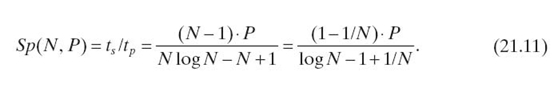
Given a platform of P cores and a chain of length N, Algorithm 21.1 leads to lower execution time than the serial exact inference if N is less than a threshold (i.e., 2^{P+ 1} for a chain of equal-size cliques); otherwise, the serial inference results in lower execution time.

Proof: When N ≤ P, we can only use N processors. Thus, we have Sp(N, P) = (N² − N)/(N log N − N + 1) ≈ N/log N, which increases as N increases. When N ≥ P, we have the following partial derivative less than 0:

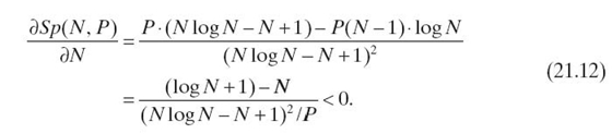
Thus, Sp(N, P) decreases monotonically as N increases when N ≥ P. By letting Equations (21.11) equal to 1, we have N ≈ 2^{P+ 1}. Thus, when N > 2^{P + 1}, Algorithm 21.1 cannot outperform a serial exact inference. When N ≫ 2^{P+ 1}, we have lim_N→∞Sp(N, P) = 0. Thus, Algorithm 21.1 leads to lower execution time than the serial exact inference only when 1 ≤ N ≤ 2^{P+ 1}. ■

Therefore, we conclude that the number of cores in a many-core processor implies a range for the number of cliques, where the proposed method shows superior performance compared with the serial exact inference. Note that the range for the number of cliques can decrease if workload is not balanced across the processors.

21.6 FROM EXACT INFERENCE TO GENERIC DIRECTED ACYCLIC GRAPH (DAG)-STRUCTURED COMPUTATIONS

We can generalize the proposed technique to some applications other than exact inference as long as the application satisfies the following constraints: (1) The application can be modeled by a DAG, where each node represents a task and the edges indicate the precedence constraints among these tasks. This is called a DAG structured computation. (2) For any adjacent tasks in the DAG, say, A → B → C, the application allows us to first partially execute task C using B that has not been updated by A, and then fully update C using A. For example, in exact inference, wecan first update the potential table of clique C using the potential table of B. As a result, the separator between B and A is brought into C to form a separator between C and A. Thus, in the next jump, C can be fully updated by A.

We generalize the proposed technique for DAG structured computations satisfying the above constraint in two steps. We first represent a given problem by a DAG. Each node in the DAG represents a set of computations on the data associated with the node. For example, in exact inference, the data associated with a node are the potential tables of the corresponding clique and the adjacent separators. The computation is to update the potential tables using node level primitives (see Section 21.2).

Second, if the DAG is not a tree or chain, we must convert it into a tree so that the proposed technique for junction trees can be used in a straightforward way. We convert a DAG into a tree as follows. We create a virtual root and connect it to all nodes without preceding nodes. There is no computation on the virtual root. Then, we identify the maximum undirected cycle in the DAG iteratively and represent each cycle as a new node. When executing a task corresponding to such a new node, we execute all the tasks in the cycle according to their original precedence constraints. Note that there is at most one preceding node for a maximum undirected cycle. This node becomes the parent of the new node. All successors of the nodes in the cycle become the children of the new node.

The above two steps convert a DAG into a tree. Due to the particular structure of a DAG, the resulting tree may or may not be suitable for pointer jumping. For example, if the undirected version of a DAG is a complete graph, the resulting tree degrades into a single node, which is not suitable for pointer jumping. The suitability of a tree for pointer jumping on parallel platforms is discussed in Section 21.5.

After we convert a DAG into a tree, we can follow Algorithm 21.1 in Section 21.4 but replace evidence propagation in lines 4 and 11 by computations associated with the corresponding nodes in the DAG. Note that Algorithm 21.1 includes two processes, bottom-up update (evidence collection) and top-down update (evidence distribution). Up on the specific application, we may only need one of the two processes. In this way, we generalize the proposed technique to some other DAG structured computations.

21.7 EXPERIMENTS

21.7.1 Platforms

We conducted experiments on two state-of-the-art many-core platforms:

• A 32-core Intel Nehalem-EX-based system consisting of four Intel Xeon X7560 processors fully connected through 6.4-GT/s QPI links. Each processor has 24-MB L3 cache and eight cores running at 2.26 GHz. All the cores share a 512-GB DDR3 memory. The operating system on this system is Red Hat Enterprise Linux Server release 5.4.
• A 24-core AMD Magny-Cours-based system consisting of two AMD Opteron 6164 HE processors. Each processor has 12-MB L3 cache and 12 cores running at 1.70 GHz. All the cores share a 64-GB DDR3 memory. The operating system on the system is CentOS Release 5.3.

21.7.2 Data Set

We evaluated the performance of our proposed algorithm using three families of junction trees: chains, balanced binary trees, and slim trees. Define junction tree width W = max_i{W_i} for a junction tree, where W_i is the number of cliques at level i of the junction tree. We call a junction tree a slim tree if it satisfies W < H, where H is the height of the tree. Note that W is an upper bound on the number of sequential evidence propagations required for updating a clique. H determines the number of pointer jumping iterations. Using slim trees, we can observe the performance of the proposed algorithm, even though there exists some amount of structural parallelism in such junction trees. The clique size, that is, the number of variables in the clique, was W_d = 12 in our experiments. This offered a limited amount of data parallelism. The random variables were set as binary, that is, r = 2, in our experiments. We utilized a junction tree of N = 6,425,610,244,096. The three different types of slim trees used in our experiments are shown in Figure 21.3. For a given N, we varied b to change slim tree topology:

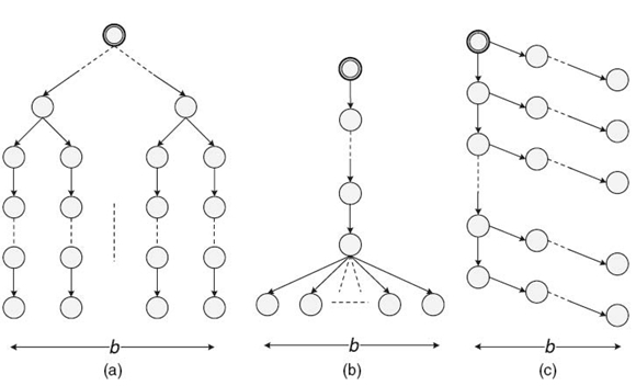
FIGURE 21.3. Three types of slim junction trees: (a) slim tree 1, (b) slim tree 2, and (c) slim tree 3.

• Slim tree 1 was formed by first creating a balanced binary tree with b leaf nodes. Then each of the leaf nodes was connected to a chain consisting of ⌈N − (2b − 1)/b⌉ nodes. The height of the tree is (⌈log b⌉ + ⌈N − (2b − 1)/b⌉). Increasing b increases the amount of structural parallelism.
• Slim tree 2 was formed by connecting b cliques to the head of a chain consisting of (N − b) nodes. The height of the tree is (N − b + 1). Increasing b increases the amount of structural parallelism. A larger b also results in more sequential operations to update a clique during evidence collection.
• Slim tree 3 was formed by first creating a chain of length ⌈N/b ⌉. Then, each clique in the chain was connected to another chain consisting of (b − 1) cliques, except that the last chain connected to the root may have less than (b − 1) cliques. The height of the tree is (⌈N/b⌉ + b − 1). Increasing b reduces the amount of structural parallelism.

21.7.3 Baseline Implementation

We use a parallel implementation as the baseline to evaluate our proposed method. The parallel implementation explores structural parallelism offered by junction trees. A collaborative scheduler proposed in Reference 13 was employed to schedule tasks to threads, where each thread was bound to a separate core. We call this baseline implementation as the scheduling-based exact inference (SEI). In this implementation, we represented a junction tree as an adjacency array, each element representing a clique and the links to the children of the clique. Each task had an attribute called the dependency degree, which was initially set as the in-degree of the corresponding clique. The scheduling activities were distributed across the threads. The adjacency array was shared by all the threads. In addition to the shared adjacency array, each clique had a ready task list to store the assigned tasks that are ready to be executed. Each core fetched a task from its ready task list and executed it locally. After the task was completed, the core reduced the dependency degree of the children of the clique. If the dependency degree of a child became 0, the child clique was assigned to the ready task list hosted by the core with the lightest workload.

21.7.4 Implementation Details

We implemented our proposed algorithm using Pthreads on many-core systems. We initiated as many threads as the number of hardware cores in the target platform. Each thread was bound to a separate core. These threads persisted over the entire program execution and communicated with each other using the shared memory.

The input junction tree was stored as an adjacency array in the memory. Similar to the SEI, the adjacency array consists of a list of nodes, each corresponding to a clique in the given junction tree. Each node has links to its children and a link to its parent. Note that the links were dynamically updated due to the nature of pointer jumping.

We define a task as the computation for updating a clique in an iteration of pointer jumping. The input to a task includes the clique to be updated and the set of cliques propagating evidence to this clique. The output of a task is the input clique after being updated. In iteration k of pointer jumping in evidence collection, a task corresponds to lines 3‒5 in Algorithm 21.1, which updates clique by sequentially performing multiple evidence propagations using cliques in ch^2k . In each iteration k of pointer jumping in evidence distribution, a task corresponds to lines 10‒11 in Algorithm 21.1, which up dates clique by performing a single evidence propagation using clique pa^2k

In each iteration of pointer jumping (in both evidence collection and evidence distribution), all of the tasks can be executed in parallel. These tasks were statically distributed to the threads by a straightforward scheme: The task corresponding to clique O ≤ i < N, is distributed to thread (i mod P), where P is the number of threads. Hence, a clique is always updated by the same thread, although the cliques propagating evidence to it vary from iteration to iteration. Note that, in an iteration, the execution time of the tasks can vary due to the different number of evidence propagations performed.

We explicitly synchronized the update operations across the threads at the end of each iteration of pointer jumping using a barrier.

21.7.5 Results

Figures 21.4‒21.6 illustrate the performance of the proposed algorithm and the SEI for various junction trees. We consider the execution time and the scalability with respect to the number of processors for each algorithm.

For chains, as shown in Figure 21.4, SEI showed limited scalability; in contrast, the proposed algorithm scaled very well with the number of cores. This is because SEI had no structural parallelism to exploit for chains. For a chain of 4096 cliques, on a single core, the proposed algorithm ran much slower than SEI; however, when the number of cores exceeded 16, the proposed algorithm ran faster than SEI.

For balanced trees, as shown in Figure 21.5, both methods scaled well due to available structural parallelism. The scalability of SEI was even better than that of the proposed algorithm. This is because for balanced trees, some cliques are updated by sequentially performing a large number of evidence propagations from its children during evidence collection in the proposed algorithm. Load imbalance can occur due to the straightforward scheduling scheme that we employed. By employing the work-sharing scheduler, SEI had better load balance. Note that SEI ran much faster than the proposed algorithm.

To better understand the impact of junction tree topology on scalability, we used slim trees for the experiments. The results are shown in Figure 21.6. The number of cliques (N) was 4096. We varied the amount of structural parallelism offered by the junction trees by changing the parameter b for each type of slim tree.

For slim tree 1, we observed that SEI did not scale when the number of cores P exceeded b. However, the proposed algorithm still scaled well since the scalability of the proposed algorithm is not significantly affected by b. Thus, when b was small and P was large, for example, b = 4 and P = 32, the proposed algorithm ran faster than SEI.

For slim tree 2, increasing b made SEI scale better. In contrast, the proposed algorithm did not scale well when b increased because of the load imbalance. Load imbalance occurs because in each iteration of pointer jumping in evidence collec-tion, some cliques are updated by sequentially performing b evidence propagations, while the other cliques perform only one evidence propagation. Thus, when b was large, for example, 256 or 1024, for the number of cores used in the experiments, SEI ran faster than the proposed algorithm. When b was small and P was large, for example, b = 16 and P = 32, the proposed algorithm ran faster than SEI.

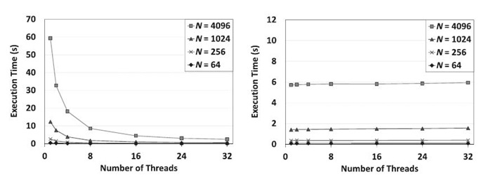
FIGURE 21.4. Comparison between the proposed algorithm (left) and SEI (right) using chains on the 32-core Intel Nehalem-EX-based system.

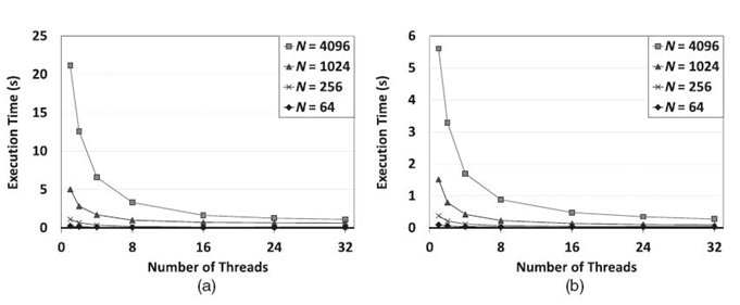
FIGURE 21.5. Comparison between the proposed algorithm (left) and SEI (right) using balanced trees on the 32-core Intel Nehalem-EX-based system.

For slim tree 3, although increasing b reduces the amount of structural parallelism, it also reduces the length of the sequential path (chains consisting of ⌈N/b⌉ cliques). Hence, as long as N/b is greater than the number of cores P, increasing b makes SEI scale better. If N/b is less than P, then all the processors are not fully utilized by SEI. We observed that, for N = 4096 and b = 256, SEI no longer scaled when the number of cores P exceeded 16. The proposed algorithm scaled best when b = 4. When b = 4 and P = 32, the proposed algorithm ran faster than SEI.

Examining the execution time of the proposed algorithm and SEI in all the cases, we can conclude that when SEI does not scale with the number of cores due to lack of structural parallelism, the proposed algorithm can offer superior performance compared with SEI by using a large number of cores.

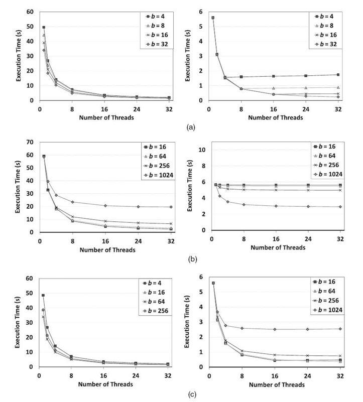
FIGURE 21.6. Comparison between the proposed algorithm and the scheduling-based exact inference (SEI) using slim trees with N = 4096 cliques on a 32-core Intel Nehalem-EX-based system. (a) The proposed algorithm (left) and SEI (right) for slim tree 1. (b) The proposed algorithm (left) and SEI (right) for slim tree 2. (c) The proposed algorithm (left) and SEI (right) for slim tree 3.

In Figures 21.7‒21.9, we illustrate the scalability of pointer jumping-based exact inference, compared with the SEI using various junction trees on a 24-core AMD Magny-Cours-based system. They correspond to the results from a 32-core Intel Nehalem-EX-based system shown in Figures 21.4‒21.6. In Figures 21.7, SEI shows no scalability since there is no structural parallelism available. However, the pointer jumping-based method worked very well. Note that, when a single core is used, the pointer jumping-based method took much more time due to the additional workload caused by pointer jumping. In Figure 21.8, the scalability of the scheduling -based method improved slightly as b increases since a large b results in higher structural parallelism at the bottom level (see Fig. 21.3b). However, since a larger b results in shorter chains, it leads to poor scalability for pointer jumping. Both methods showed scalability when using balanced trees in Figure 21.9. However, the execution time was different due to the additional workload in the pointer jumping-based method. As we can see, the results on the 24-core AMD Magny-Cours-based system are consistent to those from the 32-core Intel Nehalem-EX-based system.

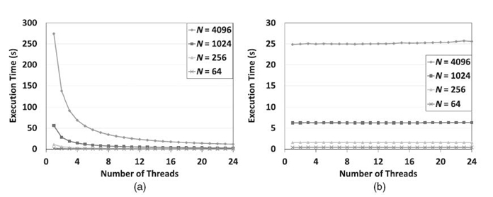
FIGURE 21.7. Comparison between the proposed method (a) and SEI (b) using chains on a 24-core AMD Magny-Cours-based system. (a) Pointer jumping-based exact inference. (b) Scheduling-based exact inference.

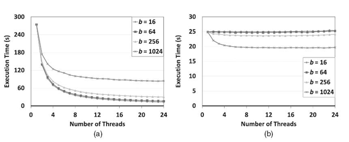
FIGURE 21.8. Comparison between the proposed method (a) and SEI (b) using slim tree 2 on a 24 -core AMD Magny-Cours based system. (a) Pointer jumping-based exact inference. (b) Scheduling -based exact inference.

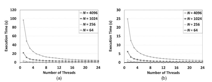
FIGURE 21.9. Comparison between the proposed method (a) and SEI (b) using balanced trees on a 24-core AMD Magny-Cours based system. (a) Pointer jumping-based exact inference. (b) Scheduling -based exact inference.

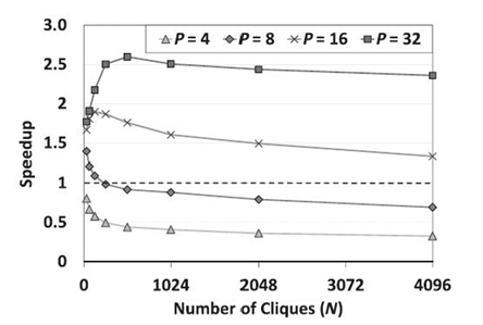
FIGURE 21.10. Speedup of pointer jumping-based exact inference with respect to serial implementation on a 32-core Intel Nehalem-EX-based system.

In Figure 21.10, we show the speedup of pointer jumping-based exact inference with respect to a serial implementation, given various numbers of cores. Sincepointer jumping-based exact inference involves additional work, it may not always outperform the scheduling-based method. We can see from Figure 21.10 that the speedup increased quickly when N was smaller than P, but then the speedup gradually decreases. When P is small, we observed that the speedup is lower than 1. This observation is consistent with our analysis in Section 21.5: Speedup can be achieved when the number of cliques in a chain (or the height of a tree) is within a range given by [1, 2 ^{P+ 1}); otherwise, the performance of pointer jumping can be adversely affected. Note that the real range can be much smaller than the above estimate due to the imbalanced workload across the levels of a tree, especially when P is small and N is large. Thus, in Figure 21.6, we can barely observe the range for P ≤ 8.

21.8 CONCLUSIONS

In this chapter, we adapted a pointer jumping-based method to explore exact inference in junction trees with limited data and structural parallelism on many-core systems. The proposed method parallelizes both evidence collection and distribution. Due to the sequential update for each clique with respect to its children, the performance of the pointer jumping-based evidence collection depends on the topology of the input junction tree. Our experimental results show that for junction trees with limited structural parallelism, the proposed algorithm is well suited for many-core platforms. In the future, we plan to improve the load balance across threads within each iteration of pointer jumping. In addition, we are considering extending the algorithm by integrating the methods exploring structural parallelism and data parallelism, so that the algorithm can automatically choose the best method for a given junction tree. We also plan to investigate the parallelization of clique update with respect to its children during evidence collection.

REFERENCES

[1] D. Sheahan, “Developing and tuning applications on UltraSPARCT1 chip multithreading systems,” Technical Report, 2007.

[2] G. Tan, V.C. Sreedhar, and G.R. Gao, “Analysis and performance results of computing betwenness centrality on IBM Cyclops64,” Journal of Supercomputing, 2009.

[3] J. JáJá, An Introduction to Parallel Algorithms. Reading, MA: Addison-Wesley, 1992.

[4] Y. Xia and V.K. Prasanna, “Parallel exact inference,” in Parallel Computing: Architectures, Algorithms and Applications, Vol. 38, Amsterdam: IOS Press, pp. 185‒192, 2007.

[5] D. Pennock, “Logarithmic time parallel Bayesian inference,” in Proceedings of the 14th Annual Conference on Uncertainty in Artificial Intelligence, pp. 431‒438, 1998.

[6] S.L. Lauritzen and D.J. Spiegelhalter, “Local computation with probabilities and graphical structures and their application to expert systems,” J. R. Stat. Soc. Ser. B, 50: 157‒224, 1988.

[7] T.H. Cormen, C.E. Leiserson, and R.L. Rivest. Introduction to Algorithms. MIT Press and McGraw-Hill, 1990.

[8] A.V. Kozlov and J.P. Singh, “A parallel Lauritzen-Spiegelhalter algorithm for probabilistic inference,” in Proceedings of Supercomputing, pp. 320‒329, 1994.

[9] Y. Xia, X. Feng, and V.K Prasanna, “Parallel evidence propagation on multicore processors,” in The 10th International Conference on Parallel Computing Technologies, pp. 377‒391, 2009.

[10] B. D'Ambrosio, T. Fountain, and Z. Li, “Parallelizing probabilistic inference: Some early explorations,” in UAI, pp. 59‒66, 1992.

[11] Y. Xia and V.K. Prasanna, “Node level primitives for parallel exact inference,” in Proceedings of the 19th International Symposium on Computer Architecture and High Performance Computing, pp. 221‒228, 2007.

[12] D.A. Bader and G. Cong, “A fast, parallel spanning tree algorithm for symmetric multiprocessors (SMPs),” Parallel and Distributed Computing, 65(9): 994‒1006, 2005.

[13] Y. Xia and V.K. Prasanna, “Collaborative scheduling of dag structured computations on multicore processors,” in CF '10: Proceedings of the 7th ACM International Conference on Computing Frontiers, pp. 63‒72, 2010.