24

–––––––––––––––––––––––

KNN Queries in Mobile Sensor Networks

Wei-Guang Teng and Kun-Ta Chuang

24.1   INTRODUCTION

Mobile sensor networks have received a significant amount of research attention in recent years because they can support a wide range of applications, for example, intelligent transportation systems (ITS) [1], wildlife conservation systems [2], and battlefield surveillance systems [3]. In most applications for sensor networks, it is expected that data on sensor nodes can be periodically queried by an external source. Important statistical information about the underlying physical processes can thus be collected for further use.

Recently, query processing techniques, including range queries, k-nearest neighbor (KNN) queries, and snapshot queries, have been widely utilized in different applications. Among the various query types for aggregating sensor information, theKNN query, which aims at finding the KNNs around a query point, q, has been recognized as one of the key spatial queries in mobile sensor networks [4–7]. Applications of KNN queries include vehicle navigation, wildlife social discovery, and squad/platoon searching on the battlefields. KNN queries can also be applied to emergency situations such as tracing the insurgents of a traffic accident, discovering the impact of a forest fire, and seeking our nearby survivors around a battlefield stronghold.

The problem of developing an efficient algorithm for a KNN search in a spatial or multidimensional database is a major research topic for various applications [8–12]. Traditional KNN query processing techniques usually assume that location data are available in a centralized database and focus on improving the index performance [5, 13–15]. However, in new applications where data sources are geographically spread(e.g., sensor networks [2, 16], wireless ad hoc networks [17], or ITS [1]), pulling data from a large number of data sources(e.g., sensor nodes, laptops, or vehicles) is usually infeasible because of high energy consumption, high communication costs, or long latencies [18,19]. Thus, for applications in mobile sensor networks, a number of studies have recently explored the so-called in-network KNN query processing techniques [9–12, 20–22]. These techniques rely on certain in-network infrastructure—index or data structures(e.g., clustered indices or spanning trees) that are distributed among the sensor nodes—to select KNN candidates, to propagate queries, and to aggregate the result.

FIGURE 24.1. Categorization of KNN query processing mechanisms.

As shown in Figure 24.1, current techniques for KNN or range query processing can be classified into two categories, that is, the centralized and the in-network approaches. Note that, in the mobile sensor network environment, the locations of the nodes may change frequently. Also, when the nodes move, the direct wireless link between the nodes and the centralized index may no longer exist. Using centralized indices may lead to substantial message routing/relay overhead. In addition, it is prohibitively expensive to maintain the up-to-date locations of moving sensors in centralized solutions. In contrast, the in-network approach does not rely on a centralized index; instead, it propagates the query directly among the sensor nodes in the network and collects relevant data to form the final result [9–12, 20–23]. This approach is favored in mobile sensor networks to prevent high energy consumption and high maintenance overhead for a centralized database.

We thus focus on the recent development of in-network KNN approaches for mobile sensor networks. Specifically, the in-network approach can be further divided into two subcategories: those relying on a certain sort of in-network infrastructure and those that are infrastructure free. The term “infrastructure” refers to a data structure distributed among the sensor nodes that is created, either once on the fly or to be updated constantly, to support the query processing. Nevertheless, the maintenance of the in-network data structure could become prohibitively costly when the sensor nodes become mobile. To eliminate this problem, infrastructure-free methods are thus proposed. The infrastructure-free methods do not rely on any precomputed network index to process queries but instead propagate a KNN query along some well-designed itineraries to collect the data [19–21]. Recently, a number of studies have addressed continuous queries using in-network techniques [5, 15, 23]. These methods are appropriate for the constant monitoring of queries of long-standing interest but are orthogonal to the on-demand queries(one time only) that we focus on in this chapter.

24.2   PRELIMINARIES AND INFRASTRUCTURE-BASED KNN QUERIES

24.2.1   Preliminaries

We give the review of the peer-tree [20], distributed spatial index(DSI) [9], KNN perimeter tree(KPT) [11, 12], density-aware itinerary-based KNN(DIKNN) [21], and parallel concentric-circle itinerary-based (PCIKNN) [22] because they are the most notable in-network frameworks for KNN queries in mobile sensor networks.

Before discussing the details of each work, we first give the formal definition of the KNN problem for sensor networks. The query that we discussed is a type of snapshot query, which is expected to obtain the query result only once during its lifetime. The KNN problem is defined as follows.

Definition 24.1 (KNN Query)   Given a set of sensor nodes S, a geographic location q (i.e., the query point), and a valid time T, find a subset S′ of S with k nodes (i.e., ) such that at time T, ∀n1 ∈ S′, n2 ∈ (S - S′): DIST(n1, q) ≤ DIST(n2 , q), where DIST denotes a distance function(usually the Euclidean distance is used).

Ideally, we expect to obtain the exact result set S′ comprising the KNNs of q at a given time T. However, because of node mobility and efficiency considerations [18, 19], we may obtain an approximate result set instead. Query result accuracy is measured by the percentage ratio of the correct KNNs (at a valid time T) that is returned. Depending on different application needs, the valid time T can be defined either as the time the query is issued or the time the result set is received.

Note that Definition 24.1 does not specify the types of information that are returned with S′. If the node order in S′ is desired, then each node may return its geolocation, and the user receiving S′ can simply determine the order of nodes by comparing their distances to the query point.

In general, the network is in the ad hoc mode, so nodes far away from their mutual coverage communicate with each other through multihops. It is expected that all of the sensor nodes are capable of storing data locally and answering the queries individually. In addition, the moving speed and directions of sensor nodes are arbitrary. Each sensor node is aware of its geolocation. Beacons with locations and identities(IDs) are periodically broadcasted. Every sensor node also maintains a table that includes IDs and locations of neighbor nodes that fall within its radio range r. Note that this network scenario complies with IEEE Standard 802.15.4 [16], in the low-rate wireless personal area network (LR-WPAN), to achieve maximum compatibility.

24.2.2  Infrastructure-Based KNN Queries

24.2.2.1   Peer-to-Peer Indexing Structure(Peer-Tree)   The peer-tree [20] is devised with a decentralized R-tree [13]. As shown in Figure 24.2, a network is partitioned into a hierarchy of minimum bounding rectangles (MBRs). Each MBR covers a geographic region that includes all of the sensor nodes that are located inside. An MBR in the higher hierarchy(say, region a in Fig. 24.2) covers all of the regions of the sub-MBRs in the child hierarchy(regions b, c, and d in Fig. 24.2). One specific node is designated as a cluster head(i.e., distributed index) in each MBR. A cluster head knows the locations and IDs of all of the other nodes within the same MBR. The cluster head also knows the locations and IDs of its parent and child cluster heads. While a 1NN(i.e., k = 1) query is issued, the source node s routes the query message to its cluster head(node E in Fig. 24.2). Upon receiving the message, the cluster head forwards the message upward in the hierarchy until the query point q is covered by the MBR of a cluster head(in this case, node A in Fig. 24.2). The cluster head then forwards the message downward in the hierarchy, looking for a child cluster head(node G in Fig. 24.2) that contains q with a minimal MBR. After that, the location of the nearest neighbor(NN) of q can be determined and the NN is informed of the query message by a unicast. Supporting the KNN queries is more complicated because it requires multiple cluster heads to find and to propagate the query message in different MBRs. Because every query message goes through the cluster heads, the major problem of these approaches is that cluster heads easily become the system bottleneck.

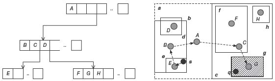
FIGURE 24.2. An example of peer-tree.

Peer-tree is the first work to utilize in-network hierarchies to maintain locations of sensor nodes. However, the solution may be vulnerable to any index failure. It is clear that there are many unnecessary hops from s to the KNN nodes because each query message is routed along the hierarchy of cluster heads, as depicted by the arrows in Figure 24.2.

24.2.2.2   DSI   Similar to peer-tree, the DSI [9] also utilizes the concept of index decentralization to maintain location information in distributed environments. DSI refers to the Hilbert curve to determine the order of objects(sensors). The basic idea is to divide all of the objects into a set of disjoint frames and to associate each frame with an index table. While linearly looking at the index table, the sensor distribution around the query point can be obtained. The major issue for the KNN search in DSI is to quickly determine a precise search space that contains k neighbors. Initially, the search space is the whole spatial area when a new KNN query is issued. The search space incrementally shrinks when a new index table is received.

Similar to peer-tree, DSI is also vulnerable to any index change. The maintenance overhead that results from the sensors moving reduces the algorithm's performance. Such overhead may become significant in the large-scale sensor networks where the distance between cluster heads is large.

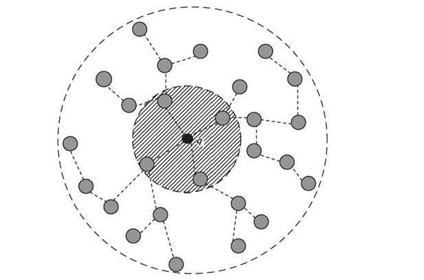
FIGURE 24.3. An example of KPT.

24.2.2.3   KNN Perimeter Tree (KPT)   To resolve the overhead in the peer-tree and DSI algorithms, the KPT algorithm [11, 12] is proposed to handle the KNN query without fixed indexing. This work assumes that each sensor node is location aware. After a query is issued from s, it is routed to the sensor node, named the home node, which is closest to q. To avoid flooding the entire network, a conservative boundary that contains at least k candidates is estimated by the home node. Multiple trees rooted at the home node are then constructed to propagate queries and to aggregate data, as shown in Figure 24.3. Upon aggregating data at the home node, the node determines the correct KNNs (by sorting locations) and transmits their query responses back to the source s.

KPT assumes an optimal network condition when each node is stationary. It encounters two serious drawbacks in the presence of mobility. First, constructing or maintaining the trees while the sensor nodes are moving incurs considerable overhead. Partially collected data may be forwarded again and again between new and old tree nodes. Second, the conservative (large) boundary grows quadratically as k increases, which leads to high energy consumption and a long latency. Although such a boundary is expected to cover at least k nodes in the worst case, sensor nodes may either move in or move out of the boundary during tree construction and data aggregation. As such, KPT is likely to return poor query results.

24.3   INFRASTRUCTURE-FREE KNN QUERIES

24.3.1   Overview of Infrastructure-Free KNN Queries

Because the maintenance overhead of infrastructure-based solutions is a critical concern when the sensor nodes are mobile, the state-of-the-art algorithms of KNN queries in mobile sensor networks thus turn to use the infrastructure-free concept when processing KNN queries [21, 22]. Currently, infrastructure-free KNN algorithms are all devised based on the itinerary-based concept. In fact, the concept of itinerary traversal is inspired by a number of research efforts in unicast routing [24], data fusion [25], network surveillance [26], and window query processing [19]. The DIKNN algorithm [21] is the first work to exploit the idea of itineraries in KNN queries for sensor networks. In general, the itinerary-based query consists of three phases: (1) the routing phase, (2) the KNN boundary estimation phase, and(3) the query dissemination and data collection phase.

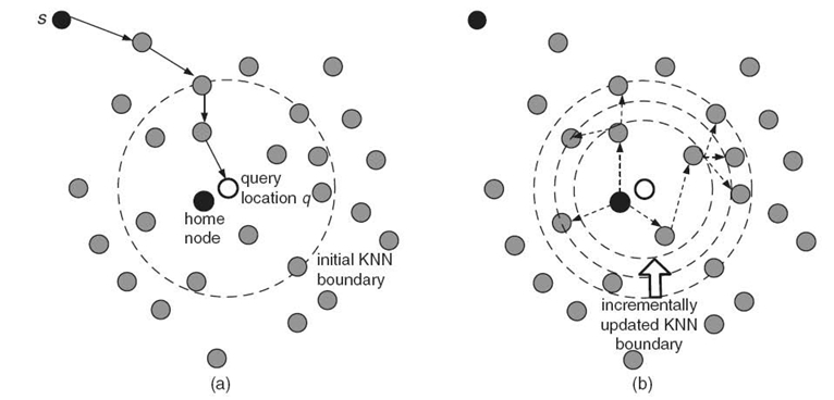
FIGURE 24.4. An illustrative example of itinerary-based KNN query processing.(a) Routing and boundary KNN estimation phases.(b) Query dissemination and data collection phase.

We show an illustrative example of an itinerary-based KNN query in Figure 24.4. Initially, a source node issues a KNN query. At the routing phase, the query is routed to the sensor node that is nearest to the query location q (such a node is referred to as the home node) by a georouting protocol such as the greedy perimeter stateless routing (GPSR) algorithm [27]. The next step, that is, the KNN boundary estimation phase, is to estimate an initial radius that can conservatively cover all of the NN sensors. The boundary can be dynamically updated during the third step of the query dissemination. The message is propagated from the home node to each node that is located within the incrementally updated KNN boundary. Finally, the query results are aggregated from the data that are collected along the itinerary of the query dissemination.

Compared to infrastructure-based algorithms, which inevitably pay for the maintenance overhead for a stable infrastructure, the itinerary-based KNN query is more feasible in a dynamic sensor network with scarce resources. Clearly, the performance, including the query latency and the energy consumption, is highly dependent on the design of the itineraries. A long itinerary traversal may lead to long query latency and high energy consumption. How to plan a good itinerary executed in the query dissemination phase is deemed as the key to the success of the itinerary-based KNN processing.

To better capture the execution of the main phase of itinerary-based KNN processing, that is, the query dissemination phase, we assume that the KNN boundary is given beforehand. Specifically, suppose that the radius of the KNN boundary is R. The home node n_p enters the query dissemination phase, aiming to inform all of the sensor nodes inside the boundary of the query message Q and to collect their responses. One naive infrastructure-tree solution is to flood the query within the boundary. Each node inside the boundary, upon receiving Q, routes its response back to s end to end and then broadcasts Q again. This approach, however, is extremely resource consuming and has poor scalability because of the excessive number of independent routing paths from sensor nodes to s [19, 21].

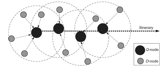
FIGURE 24.5. Various nodes in the itinerary-based query (adapted from Reference 21).

The itinerary-based dissemination technique is proposed to resolve such issues. The execution of the itinerary query dissemination can be best understood by the illustration in Figure 24.5. A set of query node s (Q-node s) in the KNN boundary is selected for the query dissemination. Upon receiving a query, a Q-node broadcasts a probe message that includes information about Q, R, and the itinerary(e.g., the itinerary width). When hearing the probe message, the neighbor nodes that are qualified to reply to the query, called data node s (D-node s), report their query response back to the Q-node. After obtaining the data from all of the D-nodes as well as the partial result that was received from the previous Q-node, the current Q-node selects the next Q-node based on the itinerary information and forwards this new partial query result to the selected next Q-node. This procedure repeats until the query traverses the entire KNN boundary along a predefined(say, spiral) itinerary structure, as shown in Figure 24.6. Responses of all nodes that are held by the last Q-node are then returned back to the sink node s in a single message.

24.3.1.1   Correctness of the Itinerary-Based Solution   The correctness of the itinerary execution has been proven in previous works [19, 21]. Formally, the itinerary width w, as shown in Figure 24.6, specifies the minimum distance between different segments of an itinerary. Obviously, a small w results in denser itinerary traversal, which ensures the KNN boundary to be fully covered by the traversal. On the other hand, the small w incurs unnecessary transmission and long latency because of the increased itinerary length. The following theorem is quoted from Reference 21.

Theorem 24.1   Let r denote the transmission range of the sensor nodes. To guarantee full coverage of a KNN boundary, the itinerary width w must be less than

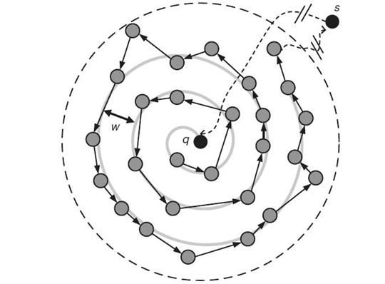
FIGURE 24.6. Itinerary-based query dissemination (adapted from Reference 21).

It can be shown [19] that letting yields full coverage while ensuring the minimal itinerary length, thus producing a good balance between query accuracy and energy efficiency. Second, data collection from multiple D-nodes must be better scheduled to avoid collisions and delays. The contention-based data collection scheme (the data collection scheme can combine both the token ring-based and the contention-based schemes to achieve higher performance [21]) can be utilized to prevent serious contention and to sustain network dynamics. In this scheme, a reference line emanating from the current Q-node is included in the probe message. The probe message also contains a precedence list indicating the reply order of D-nodes. Upon receipt of the probe message, each D-node sets a timer with timer = (α/2π)im, where α is the angle formed by the specified reference line and the line connecting the current Q-node and the current D-node, i is the received precedence, and m is a time unit for the Q-node waiting for each D-node to report its data. A D-node does not respond to the Q-node until its timer expires. Discussions on the other issues such as fault tolerance and traveling in low-connectivity areas with itinerary voids (i.e., situations when a Q-node cannot find the next Q-node for query forwarding) can be found in References 19 and 27.

In the mobile sensor network, when the Q-node moves outside the current segment during the data collection phase, it may immediately forward the partial collected results to the node nearby its original location. The data collection can be resumed on the new Q-node with a new probe message targeting only those D-nodes that did not report yet. To avoid duplicated data, each D-node can report its own ID along with the sensed data to the Q-node. By keeping the IDs of the nodes (including Q-nodes and D-nodes) collected so far in the partial query result, each Q-node is able to determine whether the coming data are duplicated or not. Note that because k is usually small, the maintenance of these IDs may not result in too much overhead.

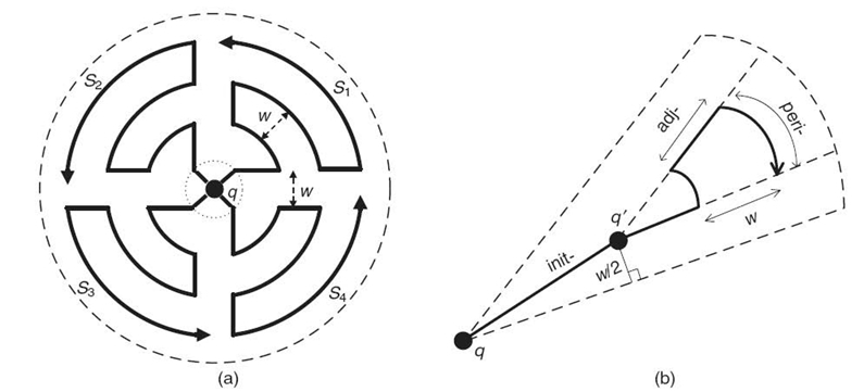
FIGURE 24.7. Concurrent query dissemination (adapted from Reference 21).(a) Concurrent itineraries.(b) Various itinerary segments.

24.3.1.2   Concurrent Itinerary Structures   Generally, the performance of dissemination solely depends on the itinerary design. Query latency can be significantly improved by considering the parallel dissemination. Nevertheless, concurrent itineraries may increase the likelihood of channel contention and collision at the data link and physical layers, causing the degradation of network throughput. Parallelization should be exercised cautiously to avoid the overhead and should satisfy the following criteria. First, the number of routing paths leading back to the sink s, after dissemination, should be controllably small to prevent high energy consumption in large-scale sensor networks. Second, as concurrent itinerary traversals may incur channel interference in wireless transmission, the chance that they meet should be as small as possible [21].

To fulfill the above criteria, a KNN boundary could be partitioned into multiple sectors, as shown in Figure 24.7 a. Such a cone-shaped itinerary is the itinerary design used in Reference 21. In each sector, the query is propagated along a subitinerary. The distance between subitineraries in adjacent sectors is w, to ensure full coverage of the KNN boundary when . Each subitinerary consists of three segments: the init-, adj-, and peri-segments, as illustrated in Figure 24.7 b. The init-segment is a portion of a subitinerary that has a distance that is less than w /2 on either side of a sector's border. This segment is formed by a straight line to reduce the interference as soon as possible.

Ideally, two subitineraries in adjacent sectors interfere with each other only at their init-segments. An important observation discussed in Reference 21 shows that even if these two subitineraries are traversed at different speeds, extra interference can only occur at adj-segments, which are relatively short as compared to peri-segments. Therefore, such a cone-shaped itinerary structure is highly adaptive to various degrees of parallelism. Note that the shape of a subitinerary degenerates into a straight line if the number of sectors is large enough. This allows for the best efficiency when no interference occurs in the sensor network(e.g., when a contention- free period [CFP] is exercised in LR-WPAN).

The concurrent itinerary traversal is a powerful functionality for the scalability issue, which has been utilized in all of the proposed itinerary-based solutions. The difference between two state-of-the-art itinerary-based algorithms lies in their design of itineraries and the corresponding KNN boundary estimation. In the following, we describe the distinguished points of two representative approaches, that is, DIKNN and PCIKNN.

24.3.2   DIKNN

24.3.2.1   KNN Boundary Estimation in DIKNN   The DIKNN algorithm [21] is the first study that employs the concept of itineraries in the KNN query processing for sensor networks. In addition to the design of itineraries, this type of algorithm also incurs a challenging issue when precisely estimating the KNN boundary. The decision of the KNN boundary must be made with very limited knowledge, which can only be obtained from query propagation. To resolve this issue, DIKNN adopts a simple and effective algorithm, named the KNN boundary(KNNB), which is tailored for sensor nodes with a limited ability.

The basic idea behind KNNB is to collect necessary information during the routing phase. In the routing phase, a query Q is routed from sink node s to the nearest neighbor n_p (i.e., the home node) around the query point q. By utilizing the geographic face routing protocol [27, 28], information collection is performed between hops. An additional list L is sent along with Q. On the ith (1 ≤ i < p) hop to the destination where p denotes the number of hops along the routing path, the corresponding node (i.e., the sensor node triggering the ith hop) appends its own location loc_i and the number of newly encountered neighbors enc_i to L. To avoid duplicate information, enc_i can simply be counted by checking the number of neighbors that have a distance larger than r from the corresponding node of the (i – 1)th hop. Note that such an information gathering technique consumes very few extra resources because only nodes around the route are involved.

Upon receipt of the query message and the list L from the previous phase, it starts estimating the KNN boundary by determining its radius length r. As described previously, too large a boundary incurs high energy consumption and a long latency. In contrast, a small boundary loses the query accuracy. The determination of r must balance two conflicting factors: (1) increasing r to enclose correct KNN points, as many as possible, and(2) decreasing r to reduce the energy consumption.

KNNB has an essential assumption: The sensor nodes are uniformly distributed within the optimal KNN boundary (i.e., the boundary containing exactly KNNs). Clearly, this assumption is easily violated when k is large. A solution to reduce the bias of estimation is also proposed. Readers can refer to the details in Reference 21.

24.3.2.2   Issues of Spatial Irregularity in DIKNN   Note that DIKNN assumes that sensor nodes are uniformly distributed around the query point q. As such, DIKNN may suffer from the issue of spatial irregularity in large-scale networks, resulting in communicacion voids and the loss of the query accuracy [29]. To handle this problem, Q-nodes in different sectors can adjust their own r during dissemination. Note that DIKNN inverses the direction of peri-segments in every interseptal sector. In such a configuration, the face-to-face adj-segments of different subitiner-aries together form rendezvous segments, in which two Q-nodes from adjacent subitineraries can, with little cost of latency, meet with each other and exchange the latest statistics. By repeating this procedure, the jth rendezvous segment in a subitinerary can obtain information from 2, 4,…, min{2j, S} nearby sectors at the j th, (j – 1)th,…, first level of the peri-segments, respectively. Each sector can thus infer how many nodes around q are explored so far (totally) and can dynamically adjust r to stop or to continue the dissemination.

24.3.2.3   Issues of Mobility Concern in DIKNN   The mobility of the sensor nodes degrades the query accuracy because the nodes may move in or move out of the KNN boundary during dissemination. For applications for which discovering correct KNNs is the most important concern, the support of flexible expansion of r to include more candidates is critical. One naive approach is to modify the KNNB algorithm so that r′ = cr′ is returned, where r′ denotes the adjusted radius of the KNN boundary and c, c > 1, denotes a constant. Obviously, for larger c, we may guarantee more correct KNNs with r′; however, more energy is consumed as well. This arrangement makes it very difficult for an application to determine a satisfactory value of c.

In DIKNN, this issue is considered in the query dissemination phase, where the last Q-node is obligated to determine how much farther a subitinerary will continue. Specifically, each application is allowed to specify an attribute, named the assurance gain g, 0 ≤ g ≤ 1, at the time when a KNN query is issued. By acquiring the moving speed of each sensor node along with its data collection, each subitinerary can maintain a record µ that specifies the fastest moving speed that was traced so far. Upon receiving this record, the last Q-node is able to measure the maximum shift of the sensor nodes by (t_s -t_e)µ, where t_s and t_e denote the time stamps of the moment the home node n_p receives the query and the query dissemination ends, respectively. Thus, an appropriate expansion of r can be obtained by r′ = r + g (t_s - t_e) µ.

To address the interaction between the mobility and spatial irregularity, it is reasonable to first adjust the KNN boundary according to the updated density information during the itinerary traversal. Afterward, a final expansion is decided (to guarantee the worst case performance) by considering the uncertainty introduced by the node mobility.

24.3.2.4   Fault Tolerance in DIKNN   Wireless sensor networks encompass various types of packet losses, which may occur because of the mobility of the sensor nodes, environmental interference, low signal-to-noise ratio s(SNR), and contentions in channel access. In DIKNN, a fault-tolerant data collection scheme is proposed. Benefiting from location awareness, a D-node receiving a probe message knows the relative reply precedence with its neighbor D-nodes. A D-node monitors (i.e., caches) its own precedence. If no acknowledgment (from the Q-node to monitored D-node) is received, then the monitoring D-node sends cached data together with its own response. This construct helps to overcome the loss of D-node responses. On the other hand, when sending the response, each D-node piggybacks the probe message upon its response so that the nearby D-nodes will have a chance to hear the probe again if the original probe from the Q-node is lost.

24.3.3   PCIKNN

Recently, a new solution, called the PCIKNN algorithm [22], has been proposed to resolve several issues found from the execution of the DIKNN algorithm. PCIKNN argues that the method for dynamic adjustment of the KNN boundary estimation in DIKNN is not always feasible in different sensor network models. In addition, determining the number of optimized KNN query threads is left unresolved for users in DIKNN.

Generally, PCIKNN also has three phases, that is, the routing phase, the KNN boundary estimation phase, and the query dissemination phase. In PCIKNN, the estimated KNN boundary can be dynamically refined while the query is propagated within the KNN boundary. Explicitly, the home node needs to collect partial results to dynamically adjust the KNN boundary. The partial data collection in the home node can also be used to guarantee that the final query result contains k-nearest nodes.

The most distinguished contribution in PCIKNN is the novel design of parallel concentric-circle itineraries, as shown in the example in Figure 24.8. The idea of parallel itineraries is first utilized in the itinerary-based query processing. Each itinerary will fork parallel threads for aggregating data in different directions. Unlike the DIKNN algorithm, which uses a single itinerary in each segment, parallel threads can help to reduce duplicated data transmissions when traversing in the inverse direction, thus leading to better power savings and improving the query latency. Furthermore, comprehensive analysis is provided to prove the model validation and to show how the PCIKNN can resist impact from spatial irregularity and mobility issues [22].

In terms of the KNN boundary estimation, DIKNN needs to record collected local information in each hop that is visited during the routing phase, which inevitably incurs extra energy overhead. To avoid energy consumption, the PCIKNN uses a linear regression technique to estimate the area that is covered by sensor nodes.

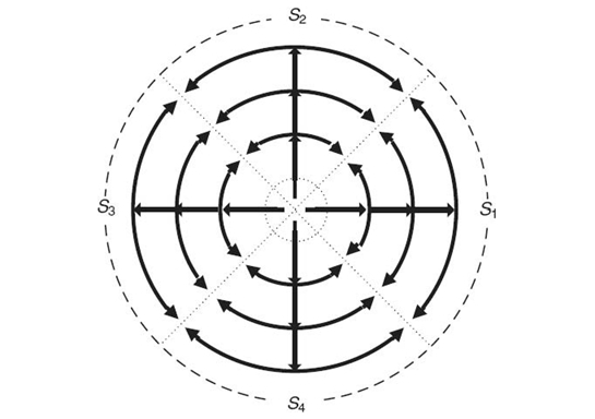
FIGURE 24.8. Parallel concentric itineraries in PCIKNN.

As reported in corresponding experimental studies [22], the regression-based solution can achieve a better boundary estimation with a relatively small energy cost.

Generally speaking, the PCIKNN algorithm uses a similar idea to handle network issues such as the mobility concern and the link failure issue. Readers can refer to the article for the discussion of such impacts on using parallel itinerary threads [22].

24.4   FUTURE RESEARCH DIRECTIONS

Query processing in mobile sensor networks remains a challenging issue. It is especially difficult to resolve the KNN issue with minimum energy consumption. Using infrastructure-based solutions will lead to prohibitively expensive maintenance overhead for index structures. On the other hand, using the infrastructure-free solution will face another critical issue when attempting to decide the KNN boundary precisely.

Currently, common research directions focus on infrastructure-free solutions because they are expected to have relatively small energy overhead(the energy issue is the most important concern in the sensor network [30]). However, we still could find some studies that demand further research, which can be summarized in the following directions.

24.4.1   Can KNN Results be Approximate?

The current KNN query processing focuses on finding precise KNN results. However, an approximate result is satisfactory in quite many applications [27]. The approximate answer is even more feasible because it is likely to be achieved at the cost of light energy consumption. Consequently, this concept would be an excellent start for further research.

24.4.2   In Addition to Itinerary-Based Solutions, Can We Have Another Way with the Infrastructure-Free Concept?

Clearly, the infrastructure-free solutions can alleviate energy concerns in mobile sensor networks. However, current solutions are all devised using itinerary traversal. Itinerary traversal inevitably faces the issues of network reliability. Even worse, duplicate data transmission cannot be completely prevented because of the node mobility. Another innovative algorithm to prevent such weaknesses under various network conditions will be a possible direction.

24.5   CONCLUSIONS

In this chapter, we have presented the status of KNN queries in mobile sensor networks. Because of its various applications, the KNN query has become one of the most important spatial queries in mobile sensor networks. We have discussed the comparison between infrastructure-based solutions and infrastructure-free solutions. To date, the itinerary-based KNN traversal, which requires no infrastructures and is able to sustain rapid changes in network topology, has been deemed as the better solution with minimum maintenance overhead and energy consumption. We have summarized possible research directions for improving current KNN queries, for example, to propose new solutions that can effectively return approximate KNN results. Finally, as technologies of sensor networks evolve, we believe that the KNN issue still requires further research effort to achieve both high precision and low power consumption.

REFERENCES

[1] U.S. Department of Transportation, “Intelligent Transportation System Joint Program Office." Available at http://www.its.dot.gov/.

[2] P. Juang, H. Oki, Y. Wang, M. Martonosi, L.S. Peh, and D. Rubenstein, “Energy-efficient computing for wildlife tracking: Design tradeoffs and early experiences with zebranet,” in Proceedings of the 10th International Conference on Architectural Support for Programming Languages and Operating Systems, pp. 96–107, 2002.

[3] Federation of American Scientists, “Remote Battlefield Sensor System(REMBASS),” 2000. Available at http://www.fas.org/man/dod-101/sys/land/rembass.htm/.

[4] H. Ferhatosmanoglu, E. Tuncel, D. Agrawal, and A.E. Abbadi, “Approximate nearest neighbor searching in multimedia databases,” in Proceedings of the 17th International Conference on Data Engineering, pp. 503–511, 2001.

[5] H.D. Chon, D. Agrawal, and A.E. Abbadi, “Range and KNN query processing for moving objects in grid model,” Mobile Networks and Applications, 8(4): 401–412, 2003.

[6] N. Roussopoulos, S. Kelley, and F. Vincent, “Nearest neighbor queries,” in Proceedings of the 1995 ACM SIGMOD International Conference on Management of Data, pp. 71–79, 1995.

[7] Z. Song and N. Roussopoulos, “K-nearest neighbor search for moving query point,” Proceedings of the 7th International Symposium on Advances in Spatial and Temporal Databases, pp. 79–96, 2001.

[8] M.-S. Chen, K.-L. Wu, and P.S. Yu, “Optimizing index allocation for sequential data broadcasting in wireless mobile computing,” IEEE Transactions on Knowledge and Data Engineering, 15(1): 161–173, 2003.

[9] W.-C. Lee and B. Zheng, “DSI: A fully distributed spatial index for location-based wireless broadcast services,” in Proceedings of the 25th IEEE International Conference on Distributed Computing Systems, pp. 349–358, 2005.

[10] B. Liu, W. Lee, and D. Lee, “Distributed caching of multi-dimensional data in mobile environments,” in Proceedings of the 6th International Conference on Mobile Data Management, pp. 229–233, 2005.

[11] J. Winter and W.-C. Lee, “KPT: A dynamic KNN query processing algorithm for location-aware sensor networks,” in Proceedings of the 1st International Workshop on Data Management for Sensor Networks, pp. 119–124, 2004.

[12] J. Winter, Y. Xu, and W.-C. Lee, “Energy efficient processing of K nearest neighbor queries in location-aware sensor networks,” in Proceedings of the 2nd Annual International Conference on Mobile and Ubiquitous Systems: Networking and Services, pp. 281–292, 2005.

[13] A. Guttman, “R-Trees: A dynamic index structure for spatial searching,” in Proceedings of the 1984 ACM SIGMOD International Conference on Management of Data, pp. 47–57, 1984.

[14] G.R. Hjaltason and H. Samet, “Distance browsing in spatial databases,” ACM Transactions on Database Systems, 24(2): 265–318, 1999.

[15] M. Mokbel, X. Xiong, and W. Aref, “SINA: Scalable incremental processing of continuous queries in spatio-temporal databases,” in Proceedings of the 2004 ACM SIGMOD International Conference on Management of Data, pp. 623–634, 2004.

[16] IEEE Standard Association, IEEE-SA 802.15.4-2003, Wireless Medium Access Control(MAC) and Physical Layer(PHY) Specifications for Low Rate Wireless Personal Area Networks. 2003.

[17] IEEE Standard Association, IEEE-SA 802.11-1997, IEEE Standard for Wireless LAN Medium Access Control(MAC) and Physical Layer(PHY) Specifications. 1997.

[18] M. Bawa, A. Gionis, H. Garcia-Molina, and R. Motwani, “The price of validity in dynamic networks,” Journal of Computer and System Sciences, 73(3): 245–264, 2007.

[19] Y. Xu, W.-C. Lee, J. Xu, and G. Mitchell, “Processing window queries in wireless sensor networks,” in Proceedings of the 22nd International Conference on Data Engineering, p.70, 2006.

[20] M. Demirbas and H. Ferhatosmanoglu, “Peer-to-peer spatial queries in sensor networks,” in Proceedings of the 3rd International Conference on Peer-to-Peer Computing, p.32, 2003.

[21] S.-H. Wu, K.-T. Chuang, C.- M. Chen, and M.- S. Chen, “Toward the optimal itinerary-based KNN query processing in mobile sensor networks,” IEEE Transactions on Knowledge and Data Engineering, 20(12): 1655–1668, 2008.

[22] T.- Y. Fu, W.-C. Peng, and W.-C. Lee, “Parallelizing itinerary-based KNN query processing in wireless sensor networks,” IEEE Transactions on Knowledge and Data Engineering, 22(5): 711–729, 2010.

[23] R. Cheng, B. Kao, S. Prabhakar, A. Kwan, and Y. Tu, “Adaptive stream filters for entity-based queries with non-value tolerance,” in Proceedings of the 31st International Conference on Very Large Data Bases, pp. 37–48, 2005.

[24] D. Niculescu and B. Nath, “Trajectory based forwarding and its applications,” in Proceedings of the 9th Annual International Conference on Mobile Computing and Networking, pp. 260–272, 2003.

[25] S. Patil, S.R. Das, and A. Nasipuri, “Serial data fusion using space-filling curves in wireless sensor networks,” in Proceedings of the 1st IEEE Communications Society Conference on Sensor and Ad Hoc Communications and Networks, pp. 182–190, 2004.

[26] C. Gui and P. Mohapatra, “Virtual patrol: A new power conservation design for surveil-lance using sensor networks,” in Proceedings of the 4th International Symposium on Information Processing in Sensor Networks, pp. 246–253, 2005.

[27] B. Karp and H. Kung, “GPSR: Greedy perimeter stateless routing for wireless networks,” in Proceedings of the 6th Annual International Conference on Mobile Computing and Networking, pp. 243–254, 2000.

[28] F. Kuhn, R. Wattenhofer, Y. Zhang, and A. Zollinger, Geometric ad-hoc routing: Of theory and practice,” in Proceedings of the 22nd Annual Symposium on Principles of Distributed Computing, pp. 63–72, 2003.

[29] D. Ganesan, S. Ratnasamy, H. Wang, and D. Estrin, “Coping with irregular spatio-temporal sampling in sensor networks,” ACM SIGCOMM Computer Communication Review, 34(1): 125–130, 2004.

[30] I.F. Akyildiz, W. Su, Y. Sankarasubramaniam, and E. Cayirci, “A survey on sensor networks,” IEEE Communications Magazine, 40(8): 102–114, 2002.