29

–––––––––––––––––––––––

Modeling of Scalable Embedded Systems

Arslan Munir, Sanjay Ranka, and Ann Gordon-Ross

29.1   INTRODUCTION

The word “embedded” literally means “within,” so embedded systems are information processing systems within (embedded into) other systems. In other words, an embedded system is a system that uses a computer to perform a specific task but is neither used nor perceived as a computer. Essentially, an embedded system is virtually any computing system other than a desktop computer. Embedded systems have links to physics and physical components, which distinguishes them from traditional desktop computing [1]. Embedded systems possess a large number of common characteristics such as real-time constraints, dependability, and power/energy efficiency.

Embedded systems can be classified based on their functionality as transformational, reactive, or interactive [2]. Transformational embedded systems take input data and transform the data into output data. Reactive embedded systems react continuously to their environment at the speed of the environment, whereas interactive embedded systems react with their environment at their own speed.

Embedded systems can be classified based on their orchestration/architecture as single-unit or multiunit embedded systems. Single-unit embedded systems refer to embedded systems that possess computational capabilities and interact with the physical world via sensors and actuators but are fabricated on a single chip and are enclosed in a single package. Multiunit embedded systems, also referred to as networked embedded systems, consist of a large number of physically distributed nodes that possess computation apabilities, interact with the physical world via a set of sensors and actuators, and communicate with each other via a wired or wireless network (since networked embedded systems are synonymous with multiunit embedded systems, we use the term multiunit embedded systems to describe these systems). Cyberphysical systems (CPSs) and wireless sensor network s (WSNs) are typical examples of multiunit embedded systems.

Interaction with the environment, timing of the operations, communication network, short time to market, and increasing customer expectations/demands for embedded system functionality have led to an exponential increase in design complexity (e.g., current automotive embedded systems contain more than 100 million lines of code). While industry focuses on increasing the number of on-chip processor cores and leveraging multiunit embedded systems to meet various application requirements, designers face an additional challenge of design scalability.

Scalability refers to the ability of a system or subsystem to be modified or adapted under varying load conditions. In other words, a system is scalable if the system's reliability and availability are within acceptable thresholds as the load or subsystems in the system increases. The scalability of a system can be classified based on geography and load [3]. A system is geographically scalable if the availability and reliability of the system are within acceptable thresholds no matter how far away the system's subsystems are located from each other. A load-scalable system exhibits acceptable availability and reliability as the load or subsystems in the system increases.

Scalability is of immense significance to embedded systems, in particular those that require several complex subsystems to work in synergy in order to accomplish a common goal (e.g., WSNs, CPSs). These systems often require adding more subsystems to the system without reengineering the existing system architecture. There are two main strategies for scaling embedded systems: scale-out and scale-up. In scale-out, which is commonly employed in multiunit embedded systems, more nodes or subsystems are added to the system (e.g., adding more sensor nodes in a WSN normally increases the sensor coverage in the sensor field as well as increases the availability and mean time to failure (MTTF) of the entire WSN due to an increase in the sensor node density). In scale-up, which is equally applicable to single-and multiunit embedded systems, more resources (e.g., computing power, memory) are added to the existing subsystems (e.g., sensor nodes can be equipped with more powerful transceivers to increase coverage).

Scalability should be distinguished from performance because these terms are related but are not synonymous (i.e., a system that scales well does not necessarily perform well). Ideally, the performance of a scalable system increases (or remains the same) and the availability increases as the system load or the number of subsystems in the system increases. The performance of an embedded system may or may not increase with scale-out or scale-in strategies. Throughput and latency are two important performance metrics for an embedded system. The throughput is the amount of work processed by a system in a given unit of time, whereas the latency is the amount of time required to complete a given task. In our WSN example, increasing the number of sensor nodes to increase situational awareness may actually decrease performance because of increased network congestion, which may increase the latency of the data delivered to a base-station node (sink node) and therefore may also delay the data processing at the sink node.

The scalability of embedded systems benefits from structured, distributed, and autonomous design. In particular, autonomous embedded systems that are able to perform data processing and decision making in situ are generally more scalable than nonautonomous embedded systems. In many applications, sensors in an embedded system generate an enormous amount of data, and limited communication bandwidth restrains the transmission of all the raw data to a central control unit. Scalability requires embedded systems/subsystems to process the information gathered from the sensors in situ and to make decisions based on the processed information. These autonomous embedded systems can scale to a very large number of nodes networked together while also reducing the need for human intervention/input by sending only concise, processed information to the network manager. To facilitate the design of scalable embedded systems with a complex design space and stringent design constraints, embedded system designers rely on various modeling paradigms.

Modeling of embedded systems helps to reduce the time to market by enabling fast application-to-device mapping, early proof of concept, and system verification. Original equipment manufacturers (OEMs) increasingly adopt model-based design methodologies for improving the quality and reuse of hardware/software (HW/SW) components. A model-based design allows development of control and dataflow applications in a graphical language familiar to control engineers and domain experts. Moreover, a model-based design enables the components'definition at a higher level of abstraction, which permits modularity and reusability. Furthermore, a model-based design allows verification of system behavior using simulation. However, different models provide different levels of abstraction for the system under design (SUD). To ensure timely completion of embedded system design with sufficient confidence in the product's market release, design engineers must make trade-offs between the abstraction level of a model and the accuracy a model can attain.

This chapter focuses on the modeling of scalable embedded systems. Section 29.2 elaborates on several embedded system application domains. Section 29.3 discusses the main components of a typical embedded system's hardware and software. Section 29.4 gives an overview of modeling, modeling objectives, and various modeling paradigms. We discuss scalability and modeling issues in single- and multiunit embedded systems along with the presentation of our work on reliability and MTTF modeling of WSNs as a modeling example in Section 29.5. Section 29.6 concludes this chapter and discusses future research directions related to the modeling of scalable embedded systems.

29.2   EMBEDDED SYSTEM APPLICATIONS

Embedded systems have applications in virtually all computing domains (except desktop computing), such as automobiles, medical, industry automation, home appliances (e.g., microwave ovens, toasters, washers/dryers), offices (e.g., printers, scanners), aircraft, space, military, and consumer electronics (e.g., smartphones, feature phones, portable media players, video games). In this section, we discuss some of these applications in detail.

29.2.1   CPSs

A CPS is an emerging application domain of multiunit embedded systems. The CPS term emphasizes the link to physical quantities, such as time, energy, and space. Although CPSs are embedded systems, this new terminology has been proposed by researchers to distinguish CPSs from simple microcontroller-based embedded systems. CPSs enable monitoring and control of physical systems via a network (e.g., Internet, Intranet, or wireless cellular network). CPSs are hybrid systems that include both continuous and discrete dynamics. Modeling of CPSs must use hybrid models that represent both continuous and discrete dynamics and should incorporate timing and concurrency. Communication between single-unit embedded devices/subsystems performing distributed computation in CPSs presents challenges due to uncertainty in temporal behavior (e.g., jitter in latency), message ordering because of dynamic routing of data, and data error rates. CPS applications include process control, networked building control systems (e.g., lighting, air-conditioning), telemedicine, and smart structures.

29.2.2   Space

Embedded systems are prevalent in space and aerospace systems where safety, reliability, and real-time requirements are critical. For example, a fly-by-wire aircraft with a 50-year production cycle requires an aircraft manufacturer to purchase, all at once, a 50-year supply of the microprocessors that will run the embedded software. All of these microprocessors must be manufactured from the same production line using the same mask to ensure that the validated, real-time performance is maintained. Consequently, aerospace systems are unable to benefit from the technological improvements in this 50-year period without repeating the software validation and certification, which is very expensive. Hence, for aerospace applications, efficiency is of less relative importance as compared to predictability and safety, which is difficult to ensure without freezing the design at the physical level [4].

Embedded systems are used in satellites and space shuttles. For example, small-scale satellites in low Earth orbit (LEO) use embedded systems for earth imaging and detection of ionospheric phenomenon that influences radio wave propagation (the ionosphere is produced by the ionization of atmospheric neutrals by ultraviolet radiation from the Sun and resides above the surface of the earth stretching from a height of 50 km to more than 1000 km) [5]. Embedded systems enable unmanned and autonomous satellite platforms for space missions. For example, the dependable multiprocessor (DM), commissioned by NASA's New Millennium Program for future space missions, is an embedded system leveraging multicore processors and field-programmable gate array (FPGA)-based coprocessors [6].

29.2.3   Medical

Embedded systems are widely used in medical equipment where a product life cycle of 7 years is a prerequisite (i.e., processors used in medical equipment must be available for at least 7 years of operation) [7]. High-performance embedded systems are used in medical imaging devices (e.g., magnetic resonance imaging (MRI), computed tomography (CT), digital X-ray, and ultrasound) to provide high-quality images, which can accurately diagnose and determine treatment for a variety of patients'conditions. Filtering noisy input data and producing high-resolution images at high data processing rates require tremendous computing power (e.g., video imaging applications often require data processing at rates of 30 images per second or more). Using multicore embedded systems helps in efficient processing of these high-resolution medical images, whereas hardware coprocessors, such as graphics processing units (GPUs) and FPGAs, take parallel computing on these images to the next step. These coprocessors off-load and accelerate some of the processing tasks that the processor would normally handle.

Some medical applications require real-time imaging to provide feedback while performing procedures, such as positioning a stent or other devices inside a patient's heart. Some imaging applications require multiple modalities (e.g., CT, MRI, ultra-sound) to provide optimal images since no single technique is optimal for imaging all types of tissues. In these applications, embedded systems combine images from each modality into a composite image that provides more information than images from each individual modality separately [8].

Embedded systems are used in cardiovascular monitoring applications to treat high-risk patients while undergoing major surgery or cardiology procedures. Hemodynamic monitors in cardiovascular embedded systems measure a range of data related to a patient's heart and blood circulation on a beat-by-beat basis. These systems monitor the arterial blood pressure waveform along with the corresponding beat durations, which determines the amount of blood pumped out with each individual beat and heart rate.

Embedded systems have made telemedicine a reality, enabling remote patient examination. Telemedicine virtually eliminates the distance between remote patients and urban practitioners by using real-time audio and video with one camera at the patient's location and another with the treatment specialist. Telemedicine requires standards-based platforms capable of integrating a myriad of medical devices via a standard I/O connection, such as Ethernet, Universal Serial Bus (USB), or video port. Vendors (e.g., Intel) supply embedded equipment for telemedicine that supports real-time transmission of high-definition audio and video while simultaneously gathering data from the attached peripheral devices (e.g., heart monitor, CT scanner, thermometer, X-ray, ultrasound machine) [9].

29.2.4   Automotive

Embedded systems are heavily used in the automotive industry for measurement and control. Since these embedded systems are commonly known as electronic control units (ECUs), we use the term ECU to refer to any automotive embedded system. A state-of-the-art luxury car contains more than 70 ECUs for safety and comfort functions [10]. Typically, ECUs in automotive systems communicate with each other over controller area network (CAN) buses.

ECUs in automotive systems are partitioned into two major categories: (1) ECUs for controlling mechanical parts and (2) ECUs for handling information systems and entertainment. The first category includes chassis control, automotive body control (interior air-conditioning, dashboard, power windows, etc.), powertrain control (engine, transmission, emissions, etc.), and active safety control. The second category includes office computing, information management, navigation, external communication, and entertainment [11]. Each category has unique requirements for computation speed, scalability, and reliability.

ECUs responsible for powertrain control, motor management, gear control, suspension control, airbag release, and antilock brakes implement closed-loop control functions as well as reactive functions with hard real-time constraints and communicate over a class C CAN bus typically operating at 1 Mbps. ECUs responsible for the powertrain have stringent real-time and computing power constraints requiring an activation period of a few milliseconds at high engine speeds. Typical powertrain ECUs use 32-bit microcontrollers running at a few hundred megahertz, whereas the remainder of the real-time subsystems use 16-bit microcontrollers running at less than 1 MHz. Multicore ECUs are envisioned as the next-generation solution for automotive applications with intense computing and high reliability requirements.

The body electronics ECUs, which serve the comfort functions (e.g., air-conditioning, power window, seat control, and parking assistance), are mainly reactive systems with only a few closed-loop control functions and have soft real-time requirements. For example, the driver and passengers issue supervisory commands to initiate power window movement by pressing the appropriate buttons. These buttons are connected to a microprocessor that translates the voltages corresponding to button up and down actions into messages that traverse over a network to the power window controller. The body electronics ECUs communicate via a class B CAN bus typically operating at 100 Kbps.

ECUs responsible for entertainment and office applications (e.g., video, sound, phone, and global positioning system [GPS]) are software intensive with millions of lines of code and communicate via an optical data bus typically operating at 100 Mbps, which is the fastest bus in automotive applications. Various CAN buses and optical buses that connect different types of ECUs in automotive applications are, in turn, connected through a central gateway, which enables the communication of all ECUs.

For high-speed communication of large volumes of data traffic generated by 360° sensors positioned around the vehicle, the automotive industry is moving toward the FlexRay communication standard (a consortium that includes BMW, DaimlerChrysler, General Motors, Freescale, NXP, Bosch, and Volkswagen/Audi as core members) [11]. The current CAN standard limits the communication speed to 500 Kbps and imposes a protocol overhead of more than 40%, whereas FlexRay defines the communication speed at 10 Mbps with comparatively less overhead than the CAN. FlexRay offers enhanced reliability using a dual-channel bus specification. The dual-channel bus configuration can exploit physical redundancy and can replicate safety-critical messages on both bus channels. The FlexRay standard affords better scalability for distributed ECUs as compared with CAN because of a time-triggered communication channel specification such that each node only needs to know the time slots for its outgoing and incoming communications. To promote high scalability, the node-assigned time slot schedule is distributed across the ECU nodes where each node stores its own time slot schedule in a local scheduling table.

29.3  EMBEDDED SYSTEMS: HARDWARE AND SOFTWARE

An interesting characteristic of embedded system design is HW/SW codesign, wherein both hardware and software must be considered together to find the appropriate combination of hardware and software that would result in the most efficient product meeting the requirement specifications. The mapping of application software to hardware must adhere to the design constraints (e.g., real-time deadlines) and objective functions (e.g., cost, energy consumption) (objective functions are discussed in detail in Section 29.4). In this section, we give an overview of embedded system hardware and software as depicted in Figure29.1.

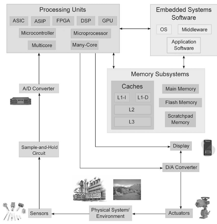
FIGURE 29.1. Embedded system hardware and software overview. A/D converter, analog-to-digital converter; D/A converter, digital-to-analog converter; ASIC, application-specifi c integrated circuit; ASIP, application-specifi c instruction set processor; FPGA, fi eld-programmable gate array; DSP, digital signal processor; GPU, graphics processing unit; OS, operating system; L1-I, level one instruction cache; L1-D, level one data cache; L2, level two unified cache; L3, level three unified cache.

29.3.1   Embedded System Hardware

Embedded system hardware is less standardized as compared to desktop computers. However, in many embedded systems, hardware is used within a loop where sensors gather information about the physical environment and generate continuous sequences of analog signals/values. Sample-and-hold circuits and analog-to-digital (A/D) converters digitize the analog signals. The digital signals are processed and the results are displayed and/or used to control the physical environment via actuators. At the output, a digital-to-analog (D/A) conversion is generally required because many actuators are analog. In the following sections, we briefly describe the hardware components of a typical embedded system [1]:

Sensors: Embedded systems contain a variety of sensors since there are sensors for virtually every physical quantity (e.g., weight, electric current, voltage, temperature, velocity, acceleration). A sensor's construction can exploit a variety of physical effects including the law of induction (voltage generation in an electric field) and photoelectric effects. Recent advances in smart embedded system design (e.g., WSNs, CPSs) can be attributed to the large variety of available sensors.

Sample-and-Hold Circuits and A/D Converters: Sample-and-hold circuits and A/D converters work in tandem to convert incoming analog signals from sensors into digital signals. Sample-and-hold circuits convert an analog signal from the continuous time domain to the discrete time domain. The circuit consists of a clocked transistor and a capacitor. The transistor functions like aswitch, where each time the switch is closed by the clocked signal, the capacitor is charged to the voltage v(t) of the incoming voltage e(t). The voltage v(t) essentially remains the same even after opening the switch because of the charge stored in the capacitor until the switch closes again. Each of the voltage values stored in the capacitor are considered as an element of a discrete sequence of values generated from the continuous signal e(t). The A/D converters map these voltage values to a discrete set of possible values afforded by the quantization process that converts these values to digits. There exists a variety of A/D converters with varying speed and precision characteristics.

Processing Units: The processing units in embedded systems process the digital signal output from the A/D converters. Energy efficiency is an important factor in the selection of processing units for embedded systems. We categorize processing units as three main types:

1. Application-Specific Integrated Circuits (ASICs). ASICs implement an embedded application's algorithm in hardware. For a fixed process technology, ASICs provide the highest energy efficiency among available processing units at the cost of no flexibility (Figure29.1).
2. Processors. Many embedded systems contain a general-purpose microprocessor and/or a microcontroller. These processors enable flexible programming but are much less energy efficient than ASICs. High-performance embedded applications leverage multicore/many-core processors, application domain-specific processors (e.g., digital signal processors [DSPs]), and application-specific instruction set processors (ASIPs) that can provide the required energy efficiency. GPUs are often used as coprocessors in imaging applications to accelerate and off-load work from the general-purpose processors (Figure29.1).
3. FPGAsSince ASICs are too expensive for low-volume applications and software-based processors can be too slow or energy inefficient, reconfigurable logic (of which FPGAs are the most prominent) can provide an energy-efficient solution. FPGAs can potentially deliver performance comparable to ASICs but offer reconfigurability using different specialized configuration data that can be used to reconfigure the device's hardware functionality. FPGAs are mainly used for hardware acceleration for low-volume applications and rapid prototyping. FPGAs can be used for rapid system prototyping that emulates the same behavior as the final system and thus can be used for experimentation purposes.

Memory Subsystems: Embedded systems require memory subsystems to store code and data. Memory subsystems in embedded systems typically consist of on-chip caches and an off-chip main memory. Caches in embedded systems are organized hierarchically: the level one instruction cache (L1-I) stores instructions; the level one data cache (L1-D) stores data; the level two unified cache (L2) stores both instructions and data; and recently, the level three unified cache (L3). Caches provide much faster access to code and data as compared to the main memory. However, caches are not suitable for real-time embedded systems because of limited predictability of hit rates and therefore access time. To offer better timing predictability for memory subsystems, many embedded systems, especially real-time embedded systems, use scratchpad memories. Scratchpad memories enable software-based control for temporary storage of calculations, data, and other work in progress instead of hardware-based control as in caches. For nonvolatile storage of code and data, embedded systems use flash memory that can be electrically erased and reprogrammed. Examples of embedded systems using flash memory include personal digital assistants (PDAs), digital audio and media players, digital cameras, mobile phones, video games, and medical equipment.

D/A Converters: Since many of the output devices are analog, embedded systems leverage D/A converters to convert digital signals to analog signals. D/A converters typically use weighted resistors to generate a current proportional to the digital number. This current is transformed into a proportional voltage by using an operational amplifier.

Output Devices: Embedded system output devices include displays and electromechanical devices known as actuators. Actuators can directly impact the environment based on the processed and/or control information from the embedded system. Actuators are key elements in reactive and interactive embedded systems, especially CPSs.

29.3.2   Embedded System Software

Embedded system software consists of an operating system (OS), middleware, and application software (Fig 29.1). Embedded software has more stringent resource constraints (e.g., smaller memory footprint, smaller data word sizes) than traditional desktop software. In the following sections, we describe an embedded system's main software components:

OS: Except for very simple embedded systems, most embedded systems require an OS for scheduling, task switching, and I/O. Embedded operating systems (EOSs) differ from traditional desktop OSs because EOSs provide limited functionality but a high level of configurability in order to accommodate a wide variety of application requirements and hardware platform features. Many embedded system applications (e.g., CPSs) are real time and require support from a real-time operating system (RTOS). An RTOS leverages deterministic scheduling policies and provides predictable timing behavior with guarantees on the upper bound of a task's execution time.

Middleware: Middleware is a software layer between the application software and the EOS. Middleware typically includes communication libraries (e.g., message-passing interface (MPI), iLib application programming interface (API) for TILERA [12]). Some real-time embedded systems require a real- time middleware.

Application Software: Embedded systems contain application software specific to the embedded application (e.g., portable media player, phone framework, health-care application, and ambient conditions monitoring application). Embedded applications leverage communication libraries provided by the middleware as well as EOS features. Application software development for embedded systems requires knowledge of the target hardware architecture because assembly language fragments are often embedded within the software code for hardware control or performance purposes. The software code is typically written in a high-level language, such as C, which promotes application software conformity to stringent resource constraints (e.g., limited memory footprint and small data word sizes).

Application software development for real-time applications must consider real-time issues, especially the worst-case execution time (WCET). The WCET is defined as the largest execution time of a program for any input and any initial execution state. We point out that the exact WCET can only be computed for certain programs and tasks such as those without recursion, without while loops, and whose loops have statically known numbers of iterations [1]. Modern pipelined processor architectures with different types of hazards (e.g., data and control hazards) and modern memory subsystems composed of different cache hierarchies with limited hit rate predictability makes WCET determination further challenging. Since exact WCET determination is extremely difficult, designers typically specify upper bounds on the WCET.

29.4   MODELING: AN INTEGRAL PART OF THE EMBEDDED SYSTEM DESIGN FLOW

Modeling stems from the concept of abstraction (i.e., defining a real-world object in a simplified form). Marwedel [1] formally defines a model as: “A model is a simplification of another entity, which can be a physical thing or another model. The model contains exactly those characteristics and properties of the modeled entity that are relevant for a given task. A model is minimal with respect to a task if it does not contain any other characteristics than those relevant for the task.”

The key phases in the embedded system design flow are requirement specifications, HW/SW partitioning, preliminary design, detailed design, component implementation, component test/validation, code generation, system integration, system verification/evaluation, and production [10]. The first phase, requirement specifications, outlines the expected/desired behavior of the SUD, and use cases describe potential applications of the SUD. Young et al. [13] commented on the importance of requirement specifications: “A design without specifications cannot be right or wrong, it can only be surprising!” HW/SW partitioning partitions an application's functionality into a combination of interacting hardware and software. Efficient and effective HW/SW partitioning can enable a product to more closely meet the requirement specifications. The preliminary design is a high-level design with minimum functionality that enables designers to analyze the key characteristics/ functionality of an SUD. The detailed design specifies the details that are absent from the preliminary design, such as detailed models or drivers for a component. Since embedded systems are complex and are composed of many components/ subsystems, many embedded systems are designed and implemented component-wise, which adds component implementation and component testing/validation phases to the design flow. Component validation may involve simulation followed by a code generation phase that generates the appropriate code for the component. System integration is the process of integrating the design of the individual components/subsystems into the complete, functioning embedded system. Verification/evaluation is the process of verifying quantitative information of key objective functions/characteristics (e.g., execution time, reliability) of a certain (possibly partial) design. Once an embedded system design has been verified, the SUD enters the production phase that produces/fabricates the SUD according to market requirements dictated by a supply-and-demand economic model. Modeling is an integral part of the embedded system design flow, which abstracts the SUD and is used throughout the design flow, from the requirement specifications phase to the formal verification/evaluation phase.

Most of the errors encountered during embedded system design are directly or indirectly related to incomplete, inconsistent, or even incorrect requirement specifications. Currently, the requirement specifications are mostly given in sentences of a natural language (e.g., English), which can be interpreted differently by the OEMs and the suppliers (e.g., Bosch or Siemens that provide embedded subsystems). To minimize the design errors, the embedded industry prefers to receive the requirement specifications in a modeling tool (e.g., graphical- or language-based). Modeling facilitates designers in deducing errors and quantitative aspects (e.g., reliability, lifetime) early in the design flow.

Once the SUD modeling is complete, the next phase is validation through simulation followed by code generation. Validation is the process of checking whether a design meets all of the constraints and performs as expected. Simulating embedded systems may require modeling the SUD, the operating environment, or both. Three terminologies are used in the literature depending on whether the SUD or the real environment or both are modeled: “Software-in-the-loop” refers to simulation where both the SUD and the real environment are modeled for early system validation; “rapid prototyping” refers to simulation where the SUD is modeled and the real environment exists for early proof of concept; and “hardware-in-the-loop” refers to simulation where the physical SUD exists and the real environment is modeled for exhaustive characterization of the SUD.

Scalability in modeling/verification means that if a modeling/verification technique can be used to abstract/verify a specific small system/subsystem, the same technique can be used to abstract/verify large systems. In some scenarios, modeling/verification is scalable if the correctness of a large system can be inferred from a small verifiable modeled system. Reduction techniques, such as partial order reduction and symmetry reduction, address this scalability problem; however, this area requires further research.

29.4.1   Modeling Objectives

Embedded system design requires characterization of several objectives, or design metrics, such as the average-case execution time and WCETs, code size, energy/ power consumption, safety, reliability, temperature/thermal behavior, electromagnetic compatibility, cost, and weight. We point out that some of these objectives can be taken as design constraints since in many optimization problems, objectives can be replaced by constraints and vice versa. Considering multiple objectives is a unique characteristic of many embedded systems and can be accurately captured using mathematical models. A system or subsystem's mathematical model is a mathematical structure consisting of sets, definitions, functions, relations, logical predicates (true or false statements), formulas, and/or graphs. Many mathematical models for embedded systems use objective function(s) to characterize some or all of these objectives, which aids in early evaluation of embedded system design by quantifying information for key objectives.

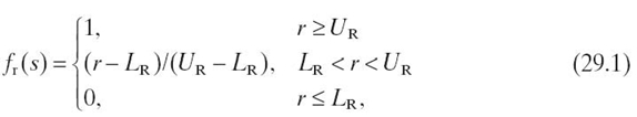
The objectives for an embedded system can be captured mathematically using linear, piecewise linear, or nonlinear functions. For example, a linear objective function for the reliability of an embedded system operating in state s (Fig 29.2) can be given as [14] where r denotes the reliability offered in the current state s (denoted as s_r in(Fig 29.2), and the constant parameters L_R and U_R denote the minimum and maximum allowed/tolerated reliability, respectively. The reliability may be represented as a multiple of a base reliability unit equal to 0.1, which represents a 10% packet reception rate [15].

Embedded systems with multiple objectives can be characterized by using either multiple objective functions, each representing a particular design metric/objective, or a single objective function that uses a weighted average of multiple objectives. A single overall objective function can be formulated as

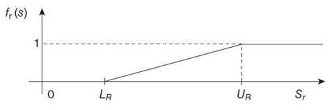
FIGURE 29.2. A linear objective function for reliability.

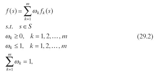
where f_k (s) and ω_k denote the objective function and weight factor for the k th objective/design metric (weight factors signify the weightage/importance of objectives with respect to each other), respectively, given that there are m objectives. Individual objectives are characterized by their respective objective functions f_k (s) (e.g., a linear objective function for reliability is given in Equation 29.1 and is depicted in Fig 29.2).

A single objective function allows selection of a single design from the design space; however, the assignment of weights for different objectives in a single objective function can be challenging using informal requirement specifications. Alternatively, the use of multiple, separate objective functions returns a set of designs from which a designer can select an appropriate design that meets the most critical objectives optimally/suboptimally. Often, embedded system modeling focuses on optimization of an objective function (e.g., power, throughput, reliability) subject to design constraints. Typical design constraints for embedded systems include safety, hard real-time requirements, and tough operating conditions in a harsh environment (e.g., aerospace), though some or all of these constraints can be added as objectives to the objective function in many optimization problems as described above.

29.4.2   Modeling Paradigms

Since embedded systems contain a large variety of abstraction levels, components, and aspects (e.g., hardware, software, functional, verification) that cannot be supported by one language or tool, designers rely on various modeling paradigms, each of which targets a partial aspect of the complete design flow from requirement specifications to production. Each modeling paradigm describes the system from a different point of view, but none of the paradigms covers all aspects. We discuss some of the modeling paradigms used in embedded system design in the following sections, each of which may use different tools to assist with modeling:

Differential Equations: Differential equation-based modeling can either use ordinary differential equations (ODEs) or partial differential equations (PDEs). ODEs (linear and nonlinear) are used to model systems or components characterized by quantities that are continuous in value and time, such as voltage and current in electrical systems, speed and force in mechanical systems, or temperature and heat flow in thermal systems [10]. ODE-based models typically describe analog electrical networks or the mechanical behavior of the complete system or component. ODEs are especially useful for studying feedback control systems that can make an unstable system stable (feedback systems measure the error [i.e., difference between the actual and desired behavior] and use this error information to correct the behavior). We emphasize that ODEs work for smooth motion where linearity, time invariance, and continuity properties hold. Nonsmooth motion involving collisions requires hybrid models that are a mixture of continuous- and discrete-time models [16].

         PDEs are used for modeling behavior in space and time, such as moving electrodes in electromagnetic fields and thermal behavior. Numerical solutions for PDEs are calculated by finite element method s (FEMs) [16].

State Machines: State machines are used for modeling discrete dynamics and are especially suitable for reactive systems. Finite-state machines (FSMs) and statecharts are some of the popular examples of state machines. Communicating finite-state machines (CFSMs) represent several FSMs communicating with each other. Statecharts extend FSMs with a mechanism for describing hierarchy and concurrency. Hierarchy is incorporated using superstates and substates, where superstates are states that comprise other substates [1]. Concurrency in statecharts is modeled using AND-states. If a system containing a superstate S is always in all of the substates of S whenever the system is in S, then the superstate S is an AND-superstate.

Dataflow: Dataflow modeling identifies and models data movement in an information system. Dataflow modeling represents processes that transform data from one form to another, external entities that receive data from a system or send data into the system, data stores that hold data, and dataflow that indicates the routes over which the data can flow. A dataflow model is represented by a directed graph where the nodes/vertices, actors, represent computation (computation maps input data streams into output data streams) and the arcs represent communication channels. Synchronous dataflow (SDF) and Kahn process networks (KPNs) are common examples of dataflow models. The key characteristics of these dataflow models is that SDFs assume that all actors execute in a single clock cycle, whereas KPNs permit actors to execute with any finite delay [1].

Discrete Event-Based Modeling: Discrete event-based modeling is based on the notion of firing or executing a sequence of discrete events, which are stored in a queue and are sorted by the time at which these events should be processed. An event corresponding to the current time is removed from the queue, processed by performing the necessary actions, and new events may be enqueued based on the action's results [1]. If there is no event in the queue for the current time, the time advances. Hardware description languages (e.g., VHDL, Verilog) are typically based on discrete event modeling. SystemC, which is a system-level modeling language, is also based on the discrete event modeling paradigm.

Stochastic Models: Numerous stochastic models exist, which mainly differ in the assumed distributions of the state residence times, to describe and analyze system performance and dependability. Analyzing an embedded system's performance in an early design phase can significantly reduce late-detected, and therefore cost-intensive, problems. Markov chains and queueing models are popular examples of stochastic models. The state residence times in Markov chains are typically assumed to have exponential distributions because exponential distributions lead to efficient numerical analysis, although other generalizations are also possible. Performance measures are obtained from Markov chains by determining steady-state and transient-state probabilities. Queueing models are used to model systems that can be associated with some notion of queues. Queueing models are stochastic models since these models represent the probability of finding a queueing system in a particular configu-ration or state.

       Stochastic models can capture the complex interactions between an embedded system and the embedded system's environment. Timeliness, concurrency, and interaction with the environment are primary characteristics of many embedded systems, and nondeterminism enables stochastic models to incorporate these characteristics. Specifically, nondeterminism is used for modeling unknown aspects of the environment or system. Markov decision processes (MDPs) are discrete stochastic dynamic programs, an extension of discrete-time Markov chains, that exhibit nondeterminism. MDPs associate a reward with each state in the Markov chain.

Petri Nets: A Petri net is a mathematical language for describing distributed systems and is represented by a directed, bipartite graph. The key elements of Petri nets are conditions, events, and a flow relation. Conditions are either satisfied or not satisfied. The flow relation describes the conditions that must be met before an event can fire as well as prescribes the conditions that become true after an event fires. Activity charts in unified modeling language (UML) are based on Petri nets [1].

29.4.3   Strategies for Integration of Modeling Paradigms

Describing different aspects and views of an entire embedded system, subsystem, or component over different development phases requires different modeling paradigms. However, sometimes, partial descriptions of a system need to be integrated for simulation and code generation. Multiparadigm languages integrate different modeling paradigms. There are two types of multiparadigm modeling [10]:

1. One model describing a system complements another model, resulting in a model of the complete system.
2. Two models give different views of the same system.

UML is an example of multiparadigm modeling, which is often used to describe software-intensive system components. UML enables the designer to verify a design before any HW/SW code is written/generated [17] and allows generation of the appropriate code for the embedded system using a set of rules. UML offers a structured and repeatable design: If there is a problem with the behavior of the application, then the model is changed accordingly, and if the problem lies in the performance of the code, then the rules are adjusted. Similarly, MATLAB's Simulink modeling environment integrates continuous-time and discrete-time models of computation based on equation solvers, a discrete event model, and an FSM model.

Two strategies for the integration of heterogeneous modeling paradigms are [10]:

1. integration of operations (analysis, synthesis) on models
2. integration of models themselves via model translation.

We briefly describe several different integration approaches that leverage these strategies in the following sections.

Cosimulation: Cosimulation permits simulation of partial models of a system in different tools and integrates the simulation process. Cosimulation depends on a central cosimulation engine, called a simulation backplane, that mediates between the distributed simulations run by the simulation engines of the participating computer-aided software engineering (CASE) tools. Cosimulation is useful and sufficient for model validation when simulation is the only purpose of model integration. In general, cosimulation is useful for the combination of a system model with a model of the system's environment since the system model is constructed completely in one tool and enters into the code generation phase, whereas the environment model is only used for simulation. Alternatively, cosimulation is insufficient if both of the models (the system and the system's environment) are intended for code generation.

Code Integration: Many modeling tools have associated code generators, and code integration is the process of integrating the generated code from multiple modeling tools. Code integration tools expedite the design process because in the absence of a code integration tool, subsystem code generated by different tools have to be integrated manually.

Code Encapsulation: Code encapsulation is a feature offered by many CASE tools that permits code encapsulation of a subsystem model as a black box in the overall system model. Code encapsulation facilitates automated code integration as well as overall system simulation.

Model Encapsulation: In model encapsulation, an original subsystem model is encapsulated as an equivalent subsystem model in the modeling language of the enclosing system. Model encapsulation permits coordinated code generation, in which the code generation for the enclosing system drives the code generator for the subsystem. The enclosing system tool can be regarded as a master tool and the encapsulated subsystem tool as a slave tool; therefore, model encapsulation requires the master tool to have knowledge of the slave tool.

Model Translation: In model translation, a subsystem model is translated syntactically and semantically to the language of the enclosing system. This translation results in a homogeneous overall system model so that one tool chain can be used for further processing of the complete system.

29.5   SINGLE- AND MULTIUNIT EMBEDDED SYSTEM MODELING

In this section, we discuss the scalability and modeling issues in single- and multiunit embedded systems. We elaborate on the modeling of scalable embedded systems using our work on reliability and MTTF modeling of WSNs [18].

29.5.1   Single-Unit Embedded Systems

A single-unit embedded system is an embedded system that contains various components (e.g., processor, memory, sensors, A/D converter) typically integrated onto a single chip and enclosed in a single package. Based on the specific application requirements, a single-unit embedded system can leverage any processor architecture, such as single-, multi-, or many-core.

As the number of cores in a single-unit multicore embedded system increases, scalability becomes a key design concern. To enhance scalability, particularly for many-core embedded systems, designers favor a distributed and structured design. Hence, cores in many-core embedded systems are typically arranged in a gridlike pattern and possess a distributed private memory and a common shared memory, similarly to TILERA's TILEPro64 [19]. The interconnection network has a signifi-cant affect on the scalability of many-core embedded systems. The interconnection network for a single-unit embedded system can contain buses, point-to-point connections, or a network-on-chip (NoC).

Buses and point-to-point connections are commonly used for single-unit embedded systems that consist of a small number of processor cores. Point-to-point and bus connections do not scale well as the number of processor cores increases because point-to-point connections suffer from an exponential increase in the number of connections between the processor cores due to the following two reasons [20]:

1. A single bus cannot provide concurrent transactions since, depending on the arbitration algorithm, access is granted to the device/component with the highest priority. Hence, bus-based interconnection networks block transactions that could potentially execute in parallel.
2. Large bus wire lengths can lead to unmanageable clock skews for large system-on-chips (SoCs) at high clock frequencies.

NoCs provide a scalable interconnection network solution for many-core embedded systems. NoCs provide higher bandwidths, higher flexibility, and solve the clock skew problems inherent in large SoCs. Inspired from the success and scalability of the Internet, NoCs use switch-based routers and packet-based communication. The following summarizes some of NoC's features that enable the NoC to scale well for many-core embedded systems [20]:

1. NoCs do not require dedicated address lines (like in bus-based interconnection networks) because NoCs use packet-based communication where the destination address is embedded in the packet header.
2. NoCs enable concurrent transactions if the network provides more than one transmission channel between a sender and a receiver.
3. NoCs eliminate clock skew issues in large SoCs because routers provide the necessary decoupling.
4. NoCs facilitate routing of wires since cores are arranged on a chip in a regular manner connected by routers and wires.

29.5.2   Multiunit Embedded Systems

Multiunit embedded systems are composed of two or more single-unit embedded systems interconnected by a wired or a wireless link. Since multiunit embedded systems consist of single-unit embedded systems, the modeling and scalability issues for single-unit embedded systems are also applicable to each constituting unit in multiunit embedded systems. Therefore, for brevity, we do not discuss the modeling and scalability issues of the single units within a multiunit embedded system. Additional scalability issues arise in multiunit embedded systems as the number of single-unit embedded systems increases. Furthermore, multiunit embedded systems present additional challenges in the design flow, particularly in modeling and verification.

Verification of multiunit embedded systems is a two-level process: single-unit verification and multiunit verification. Single-unit verification ensures that the individual embedded units work properly with well-defined interfaces that interact with the environment. Single-unit verification requires a model for the single-unit embedded system and specifications for the desired behavior. Multiunit verification ensures the correctness of the integrated system given a correct single-unit behavior. Multiunit verification requires an integrated model for the complete system, which is composed of single-unit models and the underlying communication network model.

Meeting real-time constraints in multiunit embedded systems introduces further challenges. Any real-time, multiunit embedded system requires the underlying interconnection/communication network to provide real-time guarantees for message transmissions, which is challenging given current networking technologies.

29.5.3   Reliability and MTTF Modeling of WSNs

This section presents our work on MTTF and reliability modeling of WSNs to elaborate on the modeling of scalable embedded systems with a practical modeling example. WSNs consist of spatially distributed autonomous sensor nodes that collaborate with each other to perform an application task. Figure 29.3 shows a typical WSN architecture. The sensor nodes distributed in the sensor field gather information (sensed data or statistics) about an observed phenomenon (e.g., environment, target) using attached sensors. A group of sensor nodes is called a WSN cluster. Each WSN cluster has one cluster head. Sensed data within a WSN cluster is collected by the cluster head and is relayed to a sink node (or base station) via the sensor nodes'ad hoc network. The sink node transmits the received information back to the WSN designer and/or the WSN manager via a gateway node connected to a computer network. The WSN designer is responsible for designing the WSN for a particular application to meet application requirements, such as lifetime, reliability, and throughput. After WSN design and deployment, the WSN manager manages WSN operations, such as data analysis, monitoring alive and dead sensor nodes, and alarm conditions (e.g., forest fire, volcano eruption, enemy troops).

WSN sensor nodes are typically mass produced and are often deployed in unattended and hostile environments, making them more susceptible to failures than other systems [21]. Additionally, manual inspection of faulty sensor nodes after deployment is typically impractical. Nevertheless, many WSN applications are mission critical, requiring continuous operation. Thus, in order to meet application requirements reliably, WSNs require fault detection and fault-tolerance (FT) mechanisms.

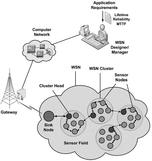
FIGURE 29.3. A typical wireless sensor network (WSN) architecture. MTTF, mean time to failure.

Fault detection encompasses distributed fault detection (DFD) algorithms that identify faulty sensor readings that indicate faulty sensors. DFD algorithms typically use existing network traffic to identify sensor failures and therefore do not incur any additional transmission cost. A fault detection algorithm's accuracy signifies the algorithm's ability to accurately identify faults. Though fault detection helps in isolating faulty sensors, WSNs require FT to reliably accomplish application tasks.

One of the most prominent FT techniques is to add hardware and/or software redundancy to the system [22]. However, WSNs are different from other systems as they have stringent constraints, and the added redundancy for FT must justify the additional cost. Studies indicate that sensors (e.g., temperature, humidity) in a sensor node have comparatively higher fault rates than other components (e.g., processors, transceivers) [23, 24]. Fortunately, sensors are cheap and adding spare sensors contributes little to the individual sensor node's cost.

29.5.3.1   FT Parameters   The FT parameters leveraged in our Markov model are coverage factor and sensor failure probability. The coverage factor c is defined as the probability that the faulty active sensor is correctly diagnosed, disconnected, and replaced by a good inactive spare sensor. The c estimation is critical in an FT WSN model and can be determined by

where c_k denotes the accuracy of the fault detection algorithm in diagnosing faulty sensors and c_c denotes the probability of an unsuccessful replacement of the identified faulty sensor with a good spare sensor. c_c depends upon the sensor switching circuitry and is usually a constant, and c_k depends upon the average number of sensor node neighbors k and the probability of sensor failure p [25, 26].

The sensor failure probability p can be represented using an exponential distribution with failure rate λ_s over the period t_s (the period t_s signifies the time over which the sensor failure probability p is specified) [27]. Thus, we can write

29.5.3.2   Fault-Tolerant Sensor Node Model   We propose an FT duplex sensor node model consisting of one active sensor (such as a temperature sensor) and one inactive spare sensor. The inactive sensor becomes active only once the active sensor is declared faulty by the fault detection algorithm. Figure29.4 shows the Markov model for our proposed FT sensor node. The states in the Markov model represent the number of good sensors. The differential equations describing the sensor node duplex Markov model are

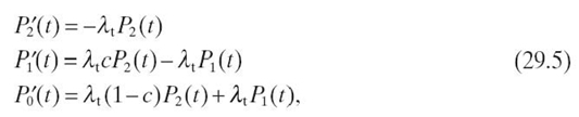
where P_i(t) denotes the probability that the sensor node will be in state i at time t and P΄_i(t) represents the first-order derivative of P_i(t).λ_t represents the failure rate of an active temperature sensor and the rate at which recoverable failure occurs is c λ_t. The probability that the sensor failure cannot be recovered is (1 − c), and the rate at which an unrecoverable failure occurs is (1 − c) λ_t.

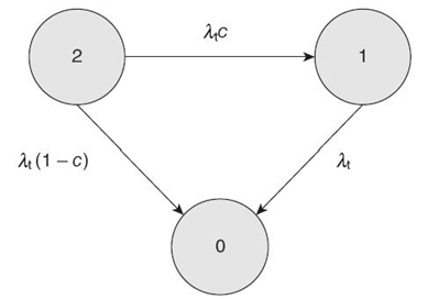
FIGURE 29.4 Sensor node Markov model.

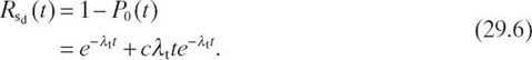
Solving Equation (29.5) with the initial conditions P₂ (0) = 1, P₁ (0) = 0, and P₀(0) = 0, the reliability of the duplex sensor node is given by

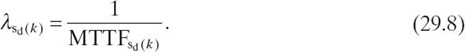
The MTTF of the duplex sensor system is

The average failure rate of the duplex sensor system depends on k (since the fault detection algorithm's accuracy depends on k [Section 29.5.3.1]) and is given by

29.5.3.3   Fault-Tolerant WSN Cluster Model   A typical WSN consists of many clusters, and we assume for our model that all nodes in a cluster are neighbors to each other. If the average number of nodes in a cluster is n, then the average number of neighbor nodes per sensor node is k = n − 1. Figure29.5 depicts our Markov model for a WSN cluster. We assume that a cluster fails (i.e., fails to perform its assigned application task) if the number of alive (nonfaulty) sensor nodes in the cluster reduces to k min. The differential equations describing the WSN cluster Markov model are

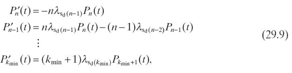
where λ_sd(n-1), λ_sd(n-2), and λ_sd(kmin) represent the duplex sensor node failure rates (Equation 29.8) when the average number of neighbor sensor nodes are n − 1, n − 2, and k_min, respectively. For mathematical tractability and closed-form solution, we analyze a special (simple) case of the above WSN cluster Markov model where n = k_min + 2, which reduces the Markov model to three states, as shown in Figure 29.6.

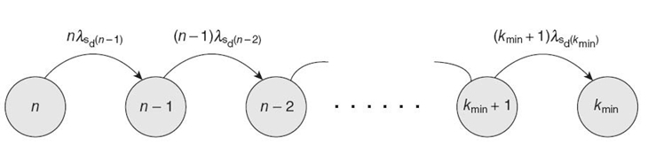
FIGURE 29.5 WSN cluster Markov model.

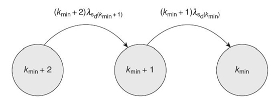
FIGURE 29.6 WSN cluster Markov model with three states.

FIGURE 29.7 WSN Markov model.

Solving Equation Equation (29.9) for n = k_{min + 2}with the initial conditions P_{kmin + 2}(0) = 1, P_{kmin + 1}(0) = 0, and P_kmin(0) = 0, the WSN cluster reliability is given as

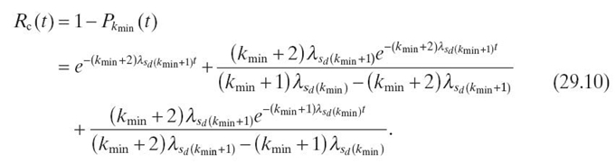
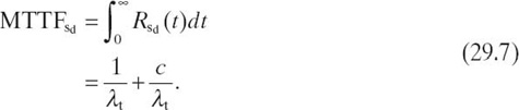
The MTTF of the WSN cluster is

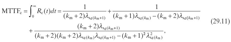
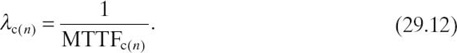
where we denote k_min by k_m in Equation (29.11) for conciseness. The average failure rate of the cluster λ_c (n) depends on the average number of nodes in cluster n at deployment time and is given by

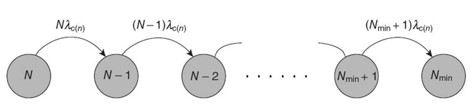
29.5.3.4   Fault-Tolerant WSN Model   A typical WSN consists of N = n_s/n clusters, where n_s denotes the total number of sensor nodes in the WSN and n denotes the average number of nodes in a cluster. Figure 29.7 depicts our WSN Markov model. We assume that the WSN fails to perform its assigned task when the number of alive clusters reduces to N_min. The differential equations describing the WSN Markov model are

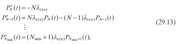
where λ_c(_n) represents the average cluster failure rate (Equation 29.12) when the cluster contains n sensor nodes at deployment time.

Solving Equation (29.13) for N = N_min + 2 with the initial conditions P_{Nmin + 2}(0) = 1, P_{Nmin + 1}(0) = 0, P_Nmin(0) = 0, the WSN reliability is given as

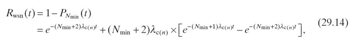
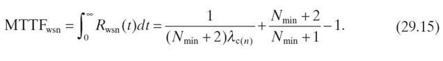
where λ_c(_n) represents the average cluster failure rate (Equation 29.12) when the cluster contains n sensor nodes at deployment time. The WSN MTTF when N = N_min + 2 is

29.5.3.5   Results and Analysis   We use the SHARPE Software Package [28] to obtain our FT sensor node, WSN cluster, and WSN model results. We assume c_c = 0 in (Equation 29.3) (i.e., once a faulty sensor is identified, the faulty sensor is replaced by a good spare sensor perfectly, and thus, c = c_k in Equation 29.3). We use typical c_k values for our analysis that represent c_k for different fault detection algorithms [25, 26]. We compare the MTTF for FT and non-fault-tolerant (NFT) sensor node, WSN cluster, and WSN models. The MTTF also reflects the system reliability (i.e., a greater MTTF implies a more reliable system).

Figure 29.8 depicts the MTTF for an NFT and FT sensor node (based on our sensor node duplex model; see Section 29.5.3.2) for k values of 5, 10, and 15 versus the sensor failure probability p when t_s in Equation (29.4) is 100 days [26]. The FT results are obtained for different k because a fault detection algorithm's accuracy, and thus c, depends upon k. The results show that the MTTF for an FT sensor node improves with increasing k. However, the MTTF shows negligible improvement when k = 15 over k = 10 as the fault detection algorithm's accuracy improvement gradient (slope) decreases between large k values. Figure 29.8 also compares the MTTF for an FT sensor node when c = 1 ∀ k, p representing the ideal case (i.e., the fault detection algorithm is perfect and the faulty sensor is identified and replaced perfectly for any number of neighbors and sensor failure probabilities). Whereas c ≠ 1 for existing fault detection algorithms, however, comparison with c = 1 provides insight into how the fault detection algorithm's accuracy affects the sensor node's MTTF. Figure 29.8 shows that the MTTF for the FT sensor node with c = 1 is always greater than the FT sensor node with c ≠ 1. We observe that the MTTF for both the NFT and FT sensor nodes decreases as p increases; however, the FT sensor node maintains better MTTF than the NFT sensor node for all p -values.

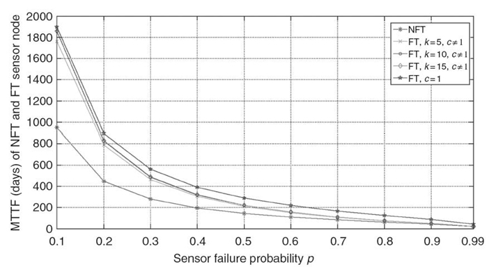
FIGURE 29.8 MTTF (days) for an FT and an NFT sensor node.

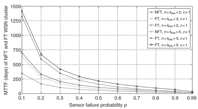
FIGURE 29.9 MTTF (days) for the FT and NFT WSN clusters with k_min = 4

Figure 29.9 depicts the MTTF for NFT and FT WSN clusters versus p when k_min = 4 (we observed similar trends for other k_min values). The FT WSN cluster consists of sensor nodes with duplex sensors (Section 29.5.3.2), and the NFT WSN cluster consists of NFT nonduplex sensor nodes. The figure shows the results for two WSN clusters that contain on average n = k_min + 2 and n = k_min + 5 sensor nodes at deployment time. The figure reveals that the FT WSN cluster's MTTF is considerably greater than the NFT WSN cluster's MTTF for both cluster systems (n = k_min + 2 and n = k_min + 5). Figure 29.9 also compares the MTTF for FT WSN clusters when c = 1 with c ≠ 1 and shows that the MTTF for FT WSN clusters with c = 1 is always better than the FT WSN clusters with c ≠ 1. We point out that both the NFT and FT WSN clusters with n > k min have redundant sensor nodes and can inherently tolerate n − k_min sensor node failures. The WSN cluster with n = k_min + 5 has more redundant sensor nodes than the WSN cluster with n = k_min + 2 and thus has a com paratively greater MTTF.

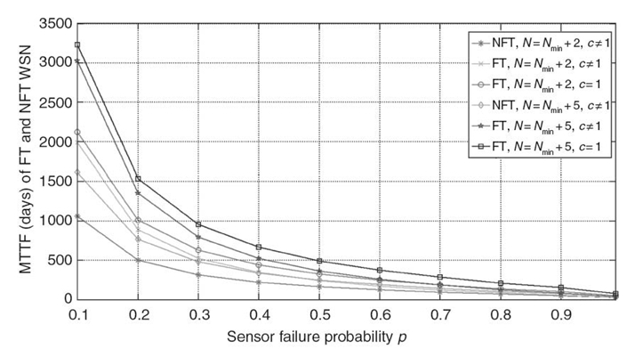
Figure 29.10 MTTF (days) for the FT and NFT WSNs with N_min = 0.

Figure 29.10 depicts the MTTF for two WSNs containing, on average, N = N_min + 2 and N = N_min + 5 clusters at deployment time, and each WSN fails when there are no more active clusters (i.e., N = N_min = 0). The FT WSN contains sensor nodes with duplex sensors (Section 29.5.3.2) and the NFT WSN contains NFT nonduplex sensor nodes. We assume that both WSNs contain clusters with n = k_min + 5, where k_min = 4 (Section 29.5.3.3). The figure reveals that the FT WSN improves the MTTF considerably over the NFT WSN for both cases (N = N_min + 2 and N = N_min + 5). Figure 29.10 also shows that the MTTF for FT WSNs when c = 1 is always greater than the MTTF for FT WSNs when c ≠ 1. We observe that as p → 1, the MTTF for the FT WSN drops close to the NFT WSN, thus leading to an important observation that, to build a more reliable FT WSN, it is crucial to have low failure probability sensors. We observe that the MTTF for WSNs with N = N_min + 5 is always greater than the MTTF for WSNs with N = N_min + 2. This observation is intuitive because WSNs with N = N_min + 5 have more redundant WSN clusters (and sensor nodes) and can survive more cluster failures before reaching the failed state (N = 0) as compared with WSNs with N = N_min + 2.

We present example reliability calculations using our Markov models for an NFT sensor node with a sensor failure rate λ_t = (− 1/100)ln(1 − 0.05) = 5.13 × 10⁻⁴ failures/day. SHARPE gives P₁(t) = e^{-5.13 × 10-4 t} and sensor node reliabil ity R_s(t). Evaluating R_s(t) at t = 100 gives R_s(t) ∣_{t = 100} = e^{-5.13 × 10-4 ×100} = 0.94999.

Using our Markov models for an FT sensor node reliability calculation when c ≠ 1, different reliability results are obtained for different k because the fault detection algorithm's accuracy and coverage factor c depends on k. For k = 5, c = 0.979, SHARPE gives P₂(t) = e^{-5.13 × 10-4 t} and P₁(t) = 5.0223 × 10^-4 te^{-5.13 × 10-4t}. The reliability R_s(t) = P₂(t) + P₁(t) = e^{-5.13 × 10-4 t} + 5.0223 × 10^-4 te^{-5.13 × 10-4 t} and R_s(t)∣_{t = 100} = e^{-5.13 × 10-4 ×100} + 5.0223 × 10^-4 ×100 ×e^{-5.13 × 10-4 ×100} = 0.94999 + 0.04771 = 0.99770.

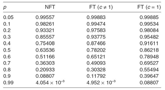
Similarly, we performed reliability calculations for an NFT and an FT WSN cluster and a complete WSN. Based on these reliability calculations, Table 29.1 shows the reliability for an NFT WSN and an FT WSN evaluated at t = 100 days when N = N_min + 2 (N_min = 0) for clusters with nine sensor nodes on average (though similar calculations can be performed for WSN clusters containing a different number of sensor nodes on average). We observe similar trends as with sensor node reliability and WSN cluster reliability, where reliability for both an NFT WSN and an FT WSN decreases as p increases (i.e., reliability R_wsn → 0 ⇔ p → 1) because a WSN contains clusters of sensor nodes, and decreased individual sensor node reliability with increasing p decreases both WSN cluster and WSN reliability. Table 29.1 shows that an FT WSN with c = 1 outperforms an FT WSN with c ≠ 1 and an NFT WSN for all p-values. For example, the percentage improvement in reliability for an FT WSN with c = 1 over an NFT WSN and an FT WSN with c ≠ 1 is 5% and 0.5% for p = 0.2 and 350% and 236% for p = 0.9, respectively. These results show that the percentage improvement in reliability attained by an FT WSN increases as p increases because the fault detection algorithm's accuracy and c decreases as p increases.

Table 29.1 Reliability for an NFT WSN and an FT When N = N_min + 2 (N_min = 0)

29.6  CONCLUSIONS

In this chapter, we discussed scalability issues in single- and multiunit embedded systems. We provided an overview of an embedded system's hardware and software components and elaborated on different applications for embedded systems with an emphasis on CPSs, space, medicine, and automotive. We discussed different approaches for modeling single- and multiunit embedded systems and the associated modeling challenges. To demonstrate the modeling of a scalable embedded system, we presented our work on reliability and MTTF modeling for WSNs. We conclude this chapter by giving future research directions related to the modeling of embedded systems.

Novel methods and tools for system-level analysis and modeling are required for embedded system design, particularly modeling tools for architecture evaluation and selection, which can profoundly impact the embedded systems'cost, performance, and quality. Further work is required in the design of modeling tools that integrate models for wireless links, which capture radio range and interference effects, in addition to the currently modeled bus-based/wired interconnection networks. Many current sensor models typically assume a circular sensing model, and there is a need to incorporate sensing irregularities in sensor models for embedded systems.

Modeling of real-time, multiunit embedded systems (e.g., CPSs) is an interesting research avenue, which requires incorporation of timing semantics in programming languages and nondeterminism in models. Memory subsystems for embedded systems, which have a profound impact on computing performance scalability, require further research to improve the timing predictability. Although scratchpad memories enable software-based control, further work is needed in this area to ensure timing guarantees. Additional research is required in networking techniques that can provide timing guarantees since current transmission control protocol/Internet protocols (TCP/IPs) are best-effort techniques over which it is extremely challenging to achieve timing predictability for real-time, multiunit embedded systems. Furthermore, network time synchronization techniques require improvement to offer better timing coherence among distributed computations.

Energy modeling for embedded systems, particularly for multiunit and many-core embedded systems, is an important research avenue. Specifically, modeling techniques to determine energy consumption for sampling sensors, packet reception, computation, and network services (e.g., routing and time synchronization) require further investigation.

ACKNOWLEDGMENTS

This work was supported by the Natural Sciences and Engineering Research Council of Canada (NSERC) and the National Science Foundation (NSF) (CNS-0905308 and CNS-0953447). Any opinions, findings, and conclusions or recommendations expressed in this material are those of the author(s) and do not necessarily reflect the views of the NSERC or NSF.

REFERENCES

[1] P. Marwedel, “Embedded and cyber-physical systems in a nutshell,” Design Automation Conference (DAC) Knowledge Center Article, November 2010.

[2] S. Edwards, L. Lavagno, E. Lee, and A. Sangiovanni-Vincentelli, “Design of embedded systems: Formal models, validation, and synthesis,” Proceedings of the IEEE, 85 (3): 366‒390, 1997.

[3] P. Sridhar, “Scalability and performance issues in deeply embedded sensor systems,” International Journal on Smart Sensing and Intelligent Systems, 2 (1): 1‒14, 2009.

[4] L. Edward, “Cyber-physical systems —Are computing foundations adequate?” NSF Workshop on Cyber-Physical Systems: Research Motivations, Techniques and Roadmap (Position Paper), Austin, TX, October 2006.

[5] G. Starr, J.M. Wersinger, R. Chapman, L. Riggs, V. Nelson, J. Klingelhoeffer, and C. Stroud, “Application of embedded systems in low Earth orbit for measurement of ionospheric anomalies,” Proceedings of the International Conference on Embedded Systems & Applications (ESA '09), Las Vegas, NV, July 2009.

[6] J. Samson, J. Ramos, A. George, M. Patel, and R. Some, “Technology validation: NMP ST8 dependable multiprocessor project,” Proceedings of the IEEE Aerospace Conference, Big Sky, MT, March 2006,

[7] Intel, “Advantech puts Intel architecture at the heart of LiDCO's advanced cardiovascular monitoring system,” in White Paper, 2010.

[8] M. Reunert, “High performance embedded systems for medical imaging,” in Intel's White Paper, October 2007.

[9] Intel, “Intel technology helps medical specialists more quickly reach —And treat — Patients in remote Areas,” in White Paper, 2011.

[10] K. Muller-Glaser, G. Frick, E. Sax, and M. Kuhl, “Multiparadigm modeling in embedded systems design,” IEEE Transactions on Control Systems Technology, 12 (2): 279‒292, 2004.

[11] A. Sangiovanni-Vincentelli and M. Natale, “Embedded system design for automotive applications,” IEEE Computer, 40 (10): 42‒51, 2007.

[12] TILERA, “TILERA multicore development environment: iLib API reference manual,” in TILERA Official Documentation, April 2009.

[13] W. Young, W. Boebert, and R. Kain, “Proving a computer system secure,” Scientific Honeyweller, 6 (2): 18‒27, 1985.

[14] A. Munir and A. Gordon-Ross, “An MDP-based dynamic optimization methodology for wireless sensor networks,” IEEE Transactions on Parallel and Distributed Systems, 23 (4): 616‒625, April 2012.

[15] J. Zhao and R. Govindan, “Understanding packet delivery performance in dense wireless sensor networks,” Proceedings of ACM SenSys, Los Angeles, CA, November 2003.

[16] C. Myers, “Modeling and verification of cyber-physical systems,” in Summer School, University of Utah, June 2011.

[17] OMG, “Unified modeling language,” in Object Management Group Standard, 2011.

[18] A. Munir and A. Gordon-Ross, “Markov modeling of fault-tolerant wireless sensor networks,” Proceedings of the IEEE International Conference on Computer Communication Networks (ICCCN), Maui, HI, August 2011.

[19] TILERA, “Manycore without boundaries: TILEPro64 processor,” July 2011.

[20] J. Henkel, W. Wolf, and S. Chakradhar, “On-chip networks: A scalable, communication - centric embedded system design paradigm,” Proceedings of the International Conference on VLSI Design (VLSID '04), Mumbai, India, January 2004.

[21] G. Werner-Allen, K. Lorincz, M. Welsh, O. Marcillo, J. Johnson, M. Ruiz, and J. Lees, “Deploying a wireless sensor network on an active volcano,” IEEE Internet Computing, 10 (2): 18‒25, 2006.

[22] I. Koren and M. Krishna, Fault-Tolerant Systems. San Francisco, CA: Morgan Kaufmann Publishers, 2007.

[23] F. Koushanfar, M. Potkonjak, and A. Sangiovanni-Vincentelli, “Fault tolerance techniques for wireless ad hoc sensor networks,” Proceedings of IEEE Sensors, Orlando, FL, June 2002.

[24] A. Sharma, L. Golubchik, and R. Govindan, “On the prevalence of sensor faults in real-world deployments,” Proceedings of the IEEE Communications Society Conference on Sensor, Mesh and Ad Hoc Communications and Networks (SECON), San Diego, CA, June 2007.

[25] P. Jiang, “A new method for node fault detection in wireless sensor networks,” Sensors, 9 (2): 1282‒1294, 2009.

[26] B. Krishnamachari and S. Iyengar, “Distributed bayesian algorithms for fault-tolerant event region detection in wireless sensor networks,” IEEE Transactions on Computers, 53 (3): 241‒250, 2004.

[27] N. Johnson, S. Kotz, and N. Balakrishnan, Continuous Univariate Distributions. New York: John Wiley and Sons, Inc., 1994.

[28] R. Sahner, K. Trivedi, and A. Puliafito, Performance and Reliability Analysis of Computer Systems: An Example-Based Approach Using the SHARPE Software Package. Dordrecht: Kluwer Academic Publishers, 1996.