32

–––––––––––––––––––––––

Dense Linear Algebra on Distributed Heterogeneous Hardware with a Symbolic DAG Approach

George Bosilca, Aurelien Bouteiller, Anthony Danalis, Thomas Herault, Piotr Luszczek, and Jack J. Dongara

32.1  INTRODUCTION AND MOTIVATION

Among the various factors that drive the momentous changes occurring in the design of microprocessors and high-end systems [1], three stand out as especially notable:

1. The number of transistors per chip will continue the current trend, that is, double roughly every 18 months, while the speed of processor clocks will cease to increase.
2. The physical limit on the number and bandwidth of the CPUs pins is becoming a near-term reality.
3. A strong drift toward hybrid/heterogeneous systems for petascale (and larger) systems is taking place.

While the first two involve fundamental physical limitations that current technology trends are unlikely to overcome in the near term, the third is an obvious consequence of the first two, combined with the economic necessity of using many thousands of computational units to scale up to petascale and larger systems.

More transistors and slower clocks require multicore designs and an increased parallelism. The fundamental laws of traditional processor design—increasing transistor density, speeding up clock rate, lowering voltage—have now been stopped by a set of physical barriers: excess heat produced, too much power consumed, too much energy leaked, and useful signal overcome by noise. Multicore designs are a natural evolutionary response to this situation. By putting multiple processor cores on a single die, architects can overcome the previous limitations and continue to increase the number of gates per chip without increasing the power densities. However, since excess heat production means that frequencies cannot be further increased, deep-and-narrow pipeline models will tend to recede as shallow-and-wide pipeline designs become the norm. Moreover, despite obvious similarities, multicore processors are not equivalent to multiple-CPUs or to symmetric multiprocessors (SMPs). Multiple cores on the same chip can share various caches (including translation look-aside buffer [TLB]) while competing for memory bandwidth. Extracting performance from such configurations of resources means that programmers must exploit increased thread-level parallelism (TLP) and efficient mechanisms for interprocessor communication and synchronization to manage resources effectively. The complexity of fine-grain parallel processing will no longer be hidden in hardware by a combination of increased instruction-level parallelism (ILP) and pipeline techniques, as it was with superscalar designs. It will have to be addressed at an upper level, in software, either directly in the context of the applications or in the programming environment. As code and performance portability remain essential, the programming environment has to drastically change.

A thicker memory wall means that communication efficiency becomes crucial. The pins that connect the processor to the main memory have become a strangle point, which, with both the rate of pin growth and the bandwidth per pin slowing down, is not flattening out. Thus, the processor-to-memory performance gap, which is already approaching a thousand cycles, is expected to grow by 50% per year according to some estimates. At the same time, the number of cores on a single chip is expected to continue to double every 18 months, and since limitations on space will keep the cache resources from growing as quickly, the cache per core ratio will continue to diminish. Problems with memory bandwidth and latency, and cache fragmentation will, therefore, tend to become more severe, and that means that communication costs will present an especially notable problem. To quantify the growing cost of communication, we can note that time per flop, network bandwidth (between parallel processors), and network latency are all improving, but at significantly different rates: 59% per year, 26% per year and 15% per year, respectively [2]. Therefore, it is expected to see a shift in algorithms’properties, from computation bound, that is, running close to peak today, toward communication bound in the near future. The same holds for communication between levels of the memory hierarchy: Memory bandwidth is improving 23% per year, and memory latency only 5.5% per year. Many familiar and widely used algorithms and libraries will become obsolete, especially dense linear algebra algorithms, which try to fully exploit all these architecture parameters. They will need to be reengineered and rewritten in order to fully exploit the power of the new architectures.

In this context, the PLASMA project [3] has developed new algorithms for dense linear algebra on shared-memory systems based on tile algorithms. Widening the scope of these algorithms from shared to distributed memory, and from homogeneous architectures to heterogeneous ones, has been the focus of a follow‒up project, DPLASMA. DPLASMA introduces a novel approach to schedule dynamically dense linear algebra algorithms on distributed systems. Similar to PLASMA, to whom it shares most of the mathematical algorithms, it is based on tile algorithms and takes advantage of DAGUE [4], a new generic distributed direct acyclic graph (DAG) engine for high-performance computing (HPC). The DAGUE engine features a DAG representation independent of the problem size, overlaps communications with computation, prioritizes tasks, schedules in an architecture-aware manner, and manages microtasks on distributed architectures featuring heterogeneous many-core nodes. The originality of this engine resides in its capability to translate a sequential nested-loop code into a concise and synthetic format, which it can interpret and then execute in a distributed environment. We consider three common dense linear algebra algorithms, namely, Cholesky, LU, and QR factorizations, part of the DPLASMA library, to investigate through the DAGUE framework their data-driven expression and execution in a distributed system. It has been demonstrated, through performance results at scale, that this approach has the potential to bridge the gap between the peak and the achieved performance that is characteristic in the state-of-the-art distributed numerical software on current and emerging architectures. However, one of the most essential contributions, in our view, is the simplicity with which new algorithmic variants may be developed and how they can be ported to a massively parallel heterogeneous architecture without much consideration, at the algorithmic level, of the underlying hardware structure or capabilities. Due to the flexibility of the underlying DAG scheduling engine and the powerful expression of parallel algorithms and data distributions, the DAGUE environment is able to deliver a significant percentage of the peak performance, providing a high level of performance portability.

32.2  DISTRIBUTED DATAFLOW BY SYMBOLIC EVALUATION

Early in the history of computing, DAGs have been used to express the dependencies between the inputs and outputs of a program’s tasks [5]. By following these dependencies, tasks whose data sets are independent (i.e., respect the Bernstein conditions [6]) can be discovered, hence enabling parallel execution. The dataflow execution model [7] is iconic of DAG-based approaches; although it has proved very successful for grid and peer-to-peer systems [8, 9], in the last two decades, it generally suffered on other HPC system types, generally because the hardware trends favored the single-program, multiple-data (SPMD) programming style with massive but uniform architectures.

Recently, the advent of multicore processors has been undermining the dominance of the SPMD programming style, reviving interest in the flexibility of dataflow approaches. Indeed, several projects [10, 14], mostly in the field of linear algebra, have proposed to revive the general use of DAGs, as an approach to tackle the challenges of harnessing the power of multicore and hybrid platforms. However, these recent projects have not considered the context of distributed-memory environments, with a massive number of many-core compute nodes clustered in a single system. In Reference 15, an implementation of a tiled algorithm based on dynamic scheduling for the LU factorization on top of Unified Parallel C (UPC) is proposed. Gustavson et al. [16] uses a static scheduling of the Cholesky factorization on top of message-passing interface (MPI) to evaluate the impact of data representation structures. All of these projects address a single problem and propose ad hoc solutions; there is clearly a need for a more ambitious framework to enable expressing a larger variety of algorithms as dataflow and to execute them on distributed systems.

Scheduling DAGs on clusters of multicores introduces new challenges: The scheduler should be dynamic to address the nondeterminism introduced by communications, and in addition to the dependencies themselves, data movements must be tracked between nodes. Evaluation of dependencies must be carried in a distributed, problem size-and system size-independent manner: The complexity of the scheduling has to be divided by the number of nodes to retain scalability at a large scale, which is not the case in many previous works that unroll the entire DAG on every compute node. Although dynamic and flexible scheduling is necessary to harness the full power of many-core nodes, network capacity is the scarcest resource, meaning that the programmer should retain control of the communication volume and pattern.

32.2.1  Symbolic Evaluation

There are three general approaches to building and managing the DAG during the execution. The first approach is to describe the DAG itself, as a potentially cyclic graph, whose set of vertices represents the tasks whose edges represent the data access dependencies. Each vertex and edge of the graph are parameterized and represent many possible tasks. At runtime, that concise representation is completely unrolled in memory, in order for the scheduling algorithm to select an ordering of the tasks that does not violate causality. The tasks are then submitted in order on the resources, according to the resulting scheduling [9]. The main drawback of this approach lies in the memory consumption associated with the complete unrolling of the DAG. Many algorithms are represented by DAGs that hold a huge number of tasks: the dense linear algebra factorizations that we use in this chapter to illustrate the DAGUE engine have a number of tasks in (n³), when the problem is of size n

The second approach is to explore the DAG according to the control flow dependency ordering given by a sequential solution to the problem [12, 14 17, 18]. The sequential code is modified with pragmas to isolate tasks that will be run as atomic entities. Every compute node then executes the sequential code in order to discover the DAG by following the sequential control flow and adding dynamic detection of the data dependency, allowing for the scheduling of tasks in parallel. Optionally, these engines use bounded buffers of tasks to limit the impact of the unrolling operation in memory. The depth of the unrolling decides the number of potential pending tasks and has a direct impact on the degree of freedom of the scheduler to find the best matched task to be scheduled. One of the central drawbacks of this approach is that a bounded buffer of tasks limits the exploration of potential parallelism according to the control flow ordering of the sequential code. Hence, it is a mixed control/dataflow approach, which is not as flexible as a true dataflow approach.

The third approach consists of using a concise, symbolic representation of the DAG at runtime. Using structures such as a parameterized task graph (PTG) proposed in Reference 19, the memory used for DAG representation is linear in the number of task types and is totally independent of the total number of tasks. At runtime, there is no a need to unroll the complete DAG, which can be explored in any order, in any direction (following a task successor or finding a task predecessor), independent of the control flow. Such a structure has been considered in Reference 20 and Reference 21, where the authors propose a centralized approach to schedule computational linear algebra tasks on clusters of SMPs using a PTG representation and remote procedure calls (RPCs).

In contrast, our approach, in DAGUE, leverages the PTG representation to evaluate the successors of a given task in a completely decentralized, distributed fashion. The IN and OUT dependencies are accessible between any pair of tasks that have a dependent relation, in the successor or predecessor direction. If task A modifies a data, d_A, and passes it to task B, task A can compute that task B is part of its successors simply by instantiating the parameters in the symbolic expression representing the dependencies of A; task B can compute that task A is part of its predecessors in the same way; and both tasks know what access type (read-write, read-only) the other tasks use on the data on this edge. Indeed, the knowledge of the IN and OUT dependencies, accessible anywhere in the DAG execution, thanks to the symbolic representation of edges, is sufficient to implement a fully distributed scheduling engine. Each node of the distributed system evaluates the successors of tasks that it has executed, only when that task completed. Hence, it never evaluates parts of the DAG pertaining to tasks executing on other resources, sparing memory and compute cycles. Not only does the symbolic representation allow the internal dependence management mechanism to efficiently compute the flow of data between tasks without having to unroll the whole DAG, but it also enables discovery of the communications required to satisfy remote dependencies, on the fly, without a centralized coordination.

As the evaluation does not rely on the control flow, the concept of algorithmic looking variants, as seen in many factorization algorithms of LAPACK and ScaLAPACK, becomes irrelevant: Instead of hard coding a particular variant of tasks ordering, such as right-looking, left-looking, or top-looking [22], the execution is now data driven; the tasks to be executed are dynamically chosen based on the resource availabilities. The issue of which “looking” variant to choose is avoided because the execution of a task is scheduled when the data are available, rather than relying on the unfolding of the sequential loops, which enables a more dynamic and flexible scheduling. However, most programmers are not used to think about the algorithm as a DAG. It is oftentimes difficult for the programmer to infer the appropriate symbolic expressions that depict the intended algorithm. We will describe in Section 32.4 how, in most cases, the symbolic representation can be simply and automatically extracted from decorated sequential code, akin to the more usual input used in code flow-based DAG engines, such as StarPU [14] and SMPSS [17]. We will then illustrate, by using the example of the QR factorization, the exact steps required from a linear algebra programmer to achieve outstanding performance on clusters of distributed heterogeneous resources, using DAGUE.

32.2.2  Task Distribution and Dynamic Scheduling

Beyond the evaluation of the DAG itself, there are a number of major principles that pertain to scheduling tasks on a distributed system. A major consideration is toward data transfers across distributed resources, in other terms, distribution of tasks across nodes and the fulfillment of remote dependencies. In many, previously cited, related projects, messaging is still explicit; the programmer has to either insert communication tasks in the DAG or insert sends and receives in the tasks themselves. As each computing node is working in its own DAG, this is equivalent to coordinating with the other DAGs using messages. This approach limits the degree of asynchrony that can be achieved by the DAG scheduling, as sends and receives have to be posted at similar time periods to avoid messaging layer resource exhaustion. Another issue is that the code tightly couples the data distribution and the algorithm. Should one decide for a new data distribution, many parts of the algorithm pertaining to communication tasks have to be modified to fit that new communication pattern.

In DAGUE, the application programmer is relieved from the low-level management: Data movements are implicit, and it is not necessary to specify how to implement the communications; they automatically overlap with computations; all computing resources (cores, accelerators, communications) of the computing nodes are handled by the DAGUE scheduler. The application developer has only to specify the data distribution as a set of immutable computable conditions. The task mapping across nodes is then mapped to the data distribution, resulting in a static distribution of tasks across nodes. This greatly alleviates the burden of the programmer who faces the complex and concurrent programming environments required for massively parallel distributed-memory machines while leaving the programmer the flexibility to address complex issues, like load balancing and communication avoidance, that are best addressed by understanding the algorithms.

This static task distribution across nodes does not mean that the overall scheduling is static. In a static scheduling, an ordering of tasks is decided offline (usually by considering the control flow of the sequential code), and resources execute tasks by strictly following that order. On the contrary, a dynamic scheduling is decided at runtime, based on the current occupation of local resources. Besides the static mapping of tasks on nodes, the order in which tasks are executed is completely dynamic. Because the symbolic evaluation of the DAG enables implicit remote dependency resolution, nodes do not need to make assumptions about the ordering of tasks on remote resources to satisfy the tight coupling of explicit send‒receive programs. As a consequence, the ordering of tasks, even those whose dependencies cross node boundaries, is completely dynamic and depends only on reactive scheduling decisions based on current network congestion and the resources available at the execution location.

When considering the additional complexity introduced by nonuniform memory hierarchies of many-core nodes and the heterogeneity from accelerators, and the desire for performance portability, it becomes clear that the scheduling must feature asynchrony and flexibility deep at its core. One of the key principles in DAGUE is the dynamic scheduling and placement of tasks within node boundaries. As soon as a resource is idling, it tries to retrieve work from other neighboring local resources in a job-stealing manner. Scheduling decisions pertaining not only to task ordering but also to resource mapping are hence completely dynamic. The programmer is relieved from the intricacies of the hardware hierarchies; his or her major role is to describe an efficient algorithm capable of expressing a high level of parallelism, and to let the DAGUE runtime take advantage of the computing capabilities of the machine and solve load imbalances that appear within nodes, automatically.

32.3  THE DAGUE DATAFLOW RUNTIME

The DAGUE engine has been designed for efficient distributed computing and has many appealing features when considering distributed-memory platforms with heterogeneous multicore nodes:

1. a symbolic dataflow representation that is independent of the problem size
2. automatic extraction of the communication from the dependencies
3. overlapping of communication and computation
4. task prioritization
5. and architecture-aware scheduling and management of tasks.

32.3.1  Intranode Dynamic Scheduling

From a technical point of view, the scheduling engine is distributively executed by all the computing resources (nodes). Its main goal is to select a local ready task for which all the IN dependencies are satisfied, that is, the data are available locally, and then to execute the body of the task on the core currently running the scheduling algorithm or on the accelerator serving this core, in the case of an accelerated-enabled kernel. Once executed, the core returns in the scheduler and releases all the OUT dependencies of this task, thus potentially making more tasks available to be scheduled, locally or remotely. It is noteworthy to mention that the scheduling mechanism is architecture aware, taking into account not only the physical layout of the cores but also the way different cache levels and memory nodes are shared between the cores. This allows the runtime to determine the best local task, that is, the one that minimizes the number of cache misses and data movements over the memory bus.

Task selection (from a list of ready to be executed tasks) is guided by a general heuristic, data locality, and a user-level controlled parameter, soft priority. The data locality policy allows the runtime to decrease the pressure on the memory bus by taking advantage of the cache locality. In Figure 32.1, two different policies of ready task management are analyzed in order to identify their impact on the task duration. The global dequeue approach manages all ready tasks in a global dequeue, shared by all threads, while the local hierarchical queue manages the ready tasks using queues shared among threads based on their distance to particular levels of memory. One can see the slight increase in the duration of the GEMM tasks when the global dequeue is used, partially due to the increased level of cache sharing between ready tasks temporarily close to each other that get executed on cores without far-apart memory sharing. At the same time, the user-defined priority is a critical component for driving the DAG execution as close as possible to the critical path, ensuring a constant high degree of parallelism while minimizing the possible starvations.

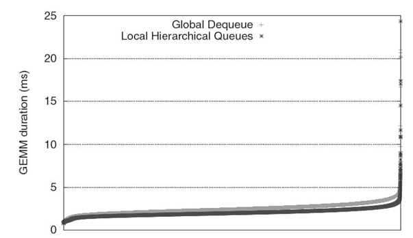
FIGURE 32.1. Duration of each individual GEMM operation in a dpotrf 10,000 × 10,000 run on 48cores (sorted by duration of the operation).

32.3.2  Communication and Data Distribution in DAGUE

The DAGUE engine is responsible for moving data from one node to another when necessary. These data movements are necessary to release dependencies of remote tasks.

The communication engine uses a type qualifier, called modifier, to define the memory layout touched by a specific data movement. Such a modifier can be expressed as MPI data types or other types of memory layout descriptors. It informs the communication engine of the shape of the data to be transferred from one memory location to another, potentially remote, memory location. The application developer is responsible for describing the type of data (by providing the above-mentioned modifier for each dataflow). At runtime, based on the data distribution, the communication engine will move the data transparently using the modifiers. The data tracking engine (described below) is capable of understanding if the different data types overlap and behaves appropriately when tracking the dependencies.

The communication engine exhibits a strong level of asynchrony in the progression of network transfers to achieve communication/computation overlap and asynchronous progress of tasks on different nodes. For that purpose, in DAGUE, communications are handled by a separate dedicated thread, which takes commands from all the other threads and issues the corresponding network operations. This thread is usually not bound on a specific core; the operating system schedules this oversubscribed thread by preempting computation-intensive threads when necessary. However, on some specific environments, due to operating system or architectural discrepancies, dedicating a hardware thread to the communication engine has been proven to be beneficial.

Upon completion of a task, the dependence resolution is executed. Local task activations are handled locally, while a task completion message is sent to processes corresponding to remote dependencies. Due to the asynchrony of the communication engine, the network congestion status does not influence the local scheduling. Thus, compute threads are able to focus on the next available compute task as soon as possible in order to maximize communication/computation overlap.

A task completion message contains information about the task that has been completed, to uniquely identify which task was completed and, consequently, to determine which data became available. Task completion messages targeting the same remote process can be coalesced, and then a single command is sent to each destination process. The successor relationship is used to build the list of processes that run tasks depending on the completed task, and these processes are then notified. The communication topology is adapted to limit the outgoing degree of one-to-all dependencies and to establish proper collective communication techniques, such as pipelining or spanning three approaches.

Upon the arrival of a task completion message, the destination process schedules the reception of the relevant output data from the parent task by evaluating, in its communication thread, the dependencies of the remote completed task. A control message is sent to the originating process to initiate the data transfers; all output data needed by the destination are received by different rendezvous messages. When one of the data transfers completes, the receiver invokes locally the dependence resolution function associated with the parent task, inside the communication thread, to release the dependencies related to this particular transfer. Remote dependency resolutions are data specific, not task specific, in order to maximize asynchrony. Tasks enabled during this process are added to the queue of the first compute thread as there are no cache constraints involved.

In the current version, the communications are performed using MPI. To increase asynchrony, data messages are nonblocking, point-to-point operations allowing tasks to concurrently release remote dependencies while keeping the maximum number of concurrent messages limited. The collaboration between the MPI processes is realized using control messages, short messages containing only the information about completed tasks. The MPI process preposts persistent receives to handle the control messages for the maximum number of concurrent task completions. Unlike data messages, there is no limit to the number of control messages that can be sent, to avoid deadlocks. This can generate unexpected messages but only for small size messages. Due to the rendezvous protocol described in the previous paragraph, the data payloads are never unexpected, thus reducing memory consumption from the network engine and ensuring flow control.

32.3.3  Accelerator Support

Accelerator computing units feature tremendous computing power, but at the expense of supplementary complexity. In large multicore nodes, load balance between the host CPU cores and the accelerators is paramount to reach a significant portion of the peak capacity of the entire node. Although accelerators usually require explicit movements of data to off-load computation to the device, considering them as mere “remote” units would not yield satisfactory results. The large discrepancy between the performance of the accelerators and the host cores renders any attempt at defining an efficient static load balance difficult. One could tune the distribution for a particular platform, but unlike data distribution among nodes, which is a generic approach to balance the load between homogeneous nodes (with potential intranode heterogeneity), static load balance for what is inherently a source of heterogeneity threatens performance portability, meaning that the code needs to be tuned, eventually significantly rewritten, for different target hardware.

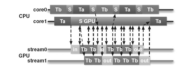
FIGURE 32.2. Schematic (not to scale) DAGUE execution on a GPU‒enabled system; kernels Ta and Tb alternate with scheduling actions (S) and in/out GPU asynchronous memory accesses.

In order to avoid these pitfalls, accelerator handling in DAGUE is dynamic and deeply integrated within the scheduler. Data movements are handled in a different manner as data movement between processes, while tasks local to the node are shared between the cores and the accelerators. In the DAGUE runtime, each thread alternates between the execution of kernels and running the lightweight scheduler (see Fig. 32.2). When an accelerator is idling and some tasks can be executed on this resource (due to the availability of an equivalent accelerator-aware kernel), the scheduler for this particular thread switches into graphics processing unit (GPU) support mode. From this point on, this thread orchestrates the data movement and submission of tasks for this GPU and remains in this mode until either the GPU queues are full or no more tasks for the GPU are available. During this period, other threads continue to operate as usual, except if additional accelerators are available. As a consequence, each GPU effectively subtracts a CPU core from the available computing power as soon as (and only if) it is processing. This cannot be avoided because the typical compute time of a GPU kernel is 10-fold smaller than a CPU one; should all CPU cores be processing, the GPU controls would be delayed to the point that would, on average, make the GPU run at the CPU speed. However, as GPU tasks are submitted asynchronously, a single CPU thread can fill all the streams of hardware supporting concurrent executions (such as NVIDIA Fermi); similarly, we investigated using a single CPU thread to manage all available accelerators, but that solution proved experimentally less scalable as the CPU processing power is overwhelmed and cannot treat the requests reactively enough to maintain all the GPUs occupied.

A significant problem introduced by GPU accelerators is data movement back and forth from the accelerator memory, which is not a share-memory space. The thread working in GPU scheduler mode multiplexes the different memory movement operations asynchronously, using multiple streams and alternating data movement orders and computation orders, to enable overlapping of I/O and GPU computation. The regular scheduling strategy of DAGUE is to favor data reuse by selecting when possible a task that reuses most of the data touched by prior tasks. The same approach is extended for the accelerator management to prioritize on the device tasks whose data have already been uploaded. Similarly, the scheduler avoids running tasks on the CPU if they depend on data that have been modified on the device (to reduce CPU/GPU data movements). A modified owned exclusive shared invalid (MOESI) [23] coherency protocol is implemented to invalidate cached data in the accelerator memory that have been updated by CPU cores. The flexibility of the symbolic representation described in Section 32.2.1 allows the scheduler to take advantage of the data proximity, a critically important feature for minimizing the data transfers to and from the accelerators. A quick look to the future tasks using a specific data provides not a prediction but a precise estimation of the interest of moving the data on the GPU.

32.4   DATAFLOW REPRESENTATION

The depiction of the data dependencies, of the task execution space, as well as the flow of data from one task to another is realized in DAGUE through an intermediary-level language named Job Data Flow (JDF). This is the representation that is at the heart of the symbolic representation of folded DAGs, allowing DAGUE to limit its memory consumption while retaining the capability of quickly finding the successors and predecessors of any given task. Figure 32.3 shows a snippet from the JDF of the linear algebra one-sided factorization QR. More details about the QR factorization and how it is fully integrated into DAGUE will be given in Section 32.5.

Figure 32.3 shows the part of the JDF that corresponds to the task class unmqr(k, n). We use the term task class to refer to a parameterized representation of a collection of tasks that all perform the same operation but on different data. Any two tasks contained in a task class are differing in their values of the parameters. In the case of unmqr (k, n), the two variables, k and n, are the parameters of this task class and, along with the ranges provided in the following two lines, define the two-dimensional (2-D) polygon that constitutes the execution space of this task class. A graphic representation of this polygon is provided by the shaded area in Figure 32.4.¹ Each lattice point included in this polygon (i.e., each point with integer coordinates) corresponds to a unique task of this task class. As implied by the term “inline_c” in the first range, the ranges of values that the parameters can take do not have to be bound by constants but can be the return value of the arbitrary C code that will be executed at runtime.

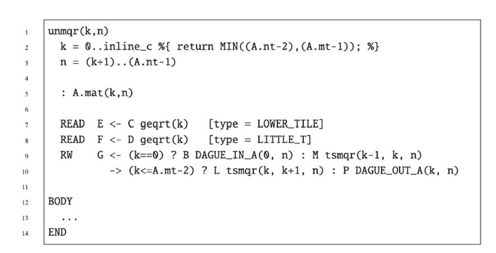
FIGURE 32.3. Sample Job Data Flow (JDF) representation.

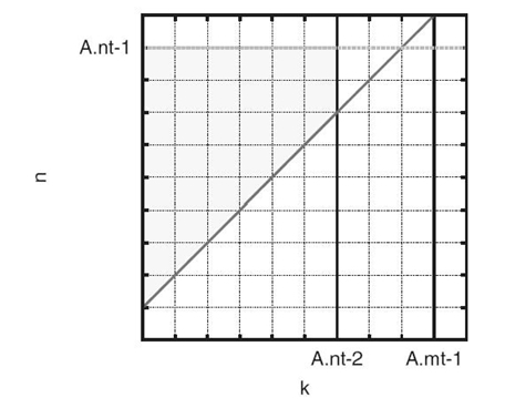
FIGURE 32.4. 2‒D Execution space of unmqr(k, n).

Below the definition of the execution space, the line

: A.mat(k, n)

defines the affinity of each task to a particular block of the data. The meaning of this notation is that the runtime must schedule task unmqr(k_i, n_i) on the node where the matrix tile A[k_i][n_i] is located, for any given values k_i and n_i. Following the affinity, there are the definitions of the dependence edges. Each line specifies an incoming or an outgoing edge. The general pattern of a line specifying a dependence edge is

(READ|WRITE|RW) IDa(<‒|‒>) [(condition) ?] IDb peer(params) [: IBc peer(params)] [type]

The keywords READ, WRITE, and RW specify if the corresponding data will be read, written, or both by the tasks of this task class. The direction of the arrow specifies that whether a given edge is input or output. A right-pointing arrow specifies an output edge, which, for this example, means that each task, unmqr (k_i, n_i), of the task class unmqr(k, n) will modify the given data, and the task (or tasks) specified on the right-hand side of the arrow will need to receive the data from task unmqr(k_i, n_i) once this task has been completed. Conversely, a left pointing arrow specifies that the corresponding data needs to be received from the task specified on the right-hand side of the arrow. The input and output identifiers (IDa and IDb) are used, in conjunction with the tasks on the two ends of an edge, to uniquely identify an edge. On the right‒hand side of each arrow, there is (1) an optional, conditional ternary operator “?: ”; (2) a unique identifier and an expression that specifies the peer task (or tasks) for this edge; and (3) an optional type specification. When a ternary operator is present, there can be one or two identifier‒task pairs as the operands of the operator. When there are two operands, the condition specifies which operand should be used as the peer task (or tasks). Otherwise, the condition specifies the values of the parameters for which the edge exists. For example, the line

RW G <-(k = = 0) ? B DAGUE_IN_A(0, n): M tsmqr(k-1, k, n)

specifies that, given specific numbers k_i and n_i, task unmqr (k_i, n_i) will receive data from task DAGUE_IN_A(0, n_i) if and only if k _i has the value zero. Otherwise, unmqr(k_i, n_i) will receive data from task tsmqr(k_i –1, k_i, n_i). Symmetrically, the JDF of task class DAGUE_IN_A(i, j) contains the following edge:

RW B -> (0 = = i) & (j > = 1) ? G unmqr(0, j)

that uniquely matches the aforementioned incoming edge of unmqr(k, n) and specifies that, for given numbers I and J, task DAGUE_IN_A(I, J) will send data to unmqr(0, J) if and only if I is equal to zero and J is greater or equal to one.

The next component of an edge specification is the task or tasks that constitute this task’s peer for this dependence edge. All the edges shown in the example of Figure 32.3 specify a single task as the peer of each task of the class unmqr(k, n) (i.e., for each specific pair of numbers k_i and n_i). The JDF syntax also allows for expressions that specify a range of tasks as the receivers of the data. Clearly, since unmqr(k, n) receives from geqrt(k) (as is specified by the first edge line in Fig. 32.3), for each value k_i, task geqrt(k_i) must send data to multiple tasks from the task class unmqr(k, n) (one for each value of n, within n’s valid range). Therefore, one of the edges of task class geqrt (k) will be as follows:

RW C -> (k< = A.nt-2) ? E unmqr(k, (k + 1)..(A.nt-1))

In this notation, the expression (k + 1)..(A.nt-1) specifies a range that guides the DAGUE runtime to broadcast the corresponding data to several receiving tasks. At first glance, it might seem that the condition “k< = A.nt-2” limiting the possible values for the parameter k in the outgoing edge of geqrt(k) (shown above) is not sufficient since it only bounds k by A.nt-2, while in the execution space of unmqr(k, n), k is also upper bound by A.mt-1. However, this additional restriction is guaranteed since the execution space of geqrt(k) (not shown here) bounds k by A.mt-1. In other words, in an effort to minimize wasted cycles at runtime, we limit the conditions that precede each edge to those that are not already covered by the conditions imposed by the execution space.

Finally, the last component of an edge specification is the type of the data exchanged during possible communications generated by this edge. This is an optional argument and it corresponds to an MPI data type, specified by the developer. The type is used to optimize the communication by avoiding the transfer of data that will not be used by the task (the data type does not have to point to a contiguous block of memory). This feature is particularly useful in cases where the operations, instead of being performed on rectangular data blocks, are applied on a part of the block, such as the upper or lower triangle in the case of QR.

Following the dependence edges, there is the body of the task class. The body specifies how the runtime can invoke the corresponding codelet that will perform the computation associated with this task class. The specifics of the body are not related to the dataflow of the problem, so they are omitted from Fig. 32.3 and are discussed in Section 32.5.

32.4.1   Starting from Sequential Source Code

Given the challenge that writing the dataflow representation can be to a nonexpert developer, a compiler tool has been developed to automatically convert an annotated C code into JDF. The analysis methodology used by our compiler is designed to only handle programs that call pure functions (no side effects) and have structured control flow. The current implementation focuses on codes written in C, with affine loop nests with array accesses and optional “if” statements. To simplify the implementation of our code analysis, we currently rely on annotations provided by the user to identify purity of functions and whether function arguments are either read or modified, or both read and modified by the function body.

Fig. 32.5 shows an example code that implements the tile QR factorization (from the PLASMA math library [12]), with minor preprocessing and simplifications performed on the code for improving readability. The code consists of four imperfectly nested loops with a maximum nesting depth of three. In the body of each loop, there are calls to the kernels that implement the four mathematical operations that constitute the QR factorization: geqrt, unmqr, tsqrt, and tsmqr (more details will be given in Section 32.5.1). The data matrices “A” and “T” are organized in tiles, and notations such as “A[m][k]” refer to a block of data (a tile) and not a single element of the matrix. We chose to use PLASMA code as our input for several reasons. First, the linear algebra operations that are implemented in PLASMA are important to the scientific community. Second, the application programming interface (API) of PLASMA includes hints that function as annotations that can help compiler analysis. In particular, for every parameter passed to a kernel, which corresponds to a matrix tile, the parameter that follows it specifies whether this tile is read, modified, or both, using the special values INPUT, OUTPUT, and INOUT, or if it is temporary, locally allocated SCRATCH memory. Further keywords specify if only a part of a tile is read, or modified, which can reduce unnecessary dependencies between kernels and increase available parallelism. Finally, all PLASMA kernels are side-effect free. This means that they operate on, and potentially change, only memory pointed to by their arguments. Also, this memory does not contain overlapping regions; that is, the arguments are not aliased.

These facts are important because they eliminate the need for interprocedural analysis or additional annotations. In other words, DAGUE’s compiler can process PLASMA code without requiring human intervention. However, the analysis performed by the compiler is not limited in any way to PLASMA codes and can accept any code for which some form of annotations (or interprocedural analysis) has provided the behavior of the functions with respect to their arguments as well as a guarantee that the functions are side-effect free.

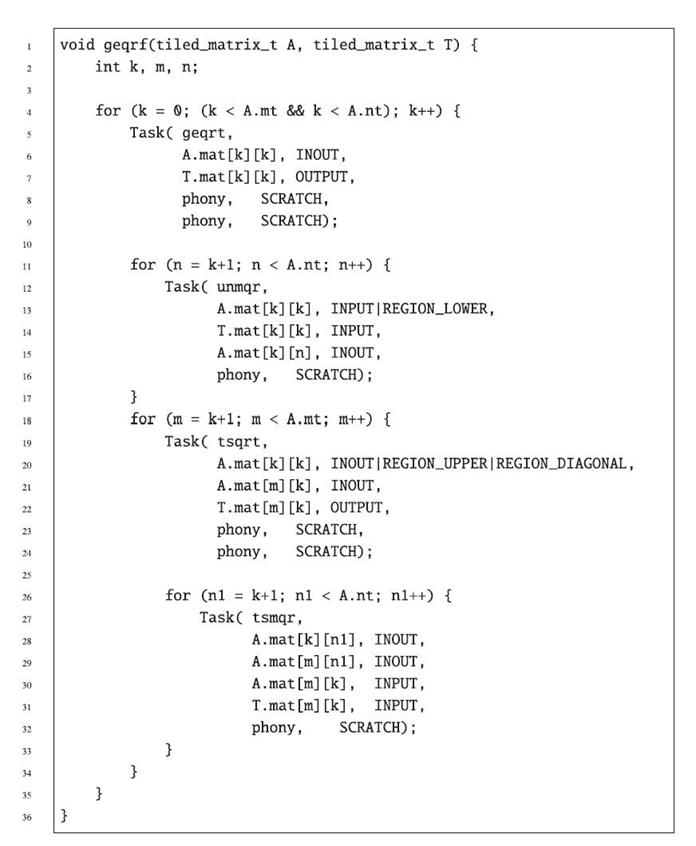
FIGURE 32.5. Tile QR factorization in PLASMA.

32.4.2   Conditional Dataflow

As stated previously, the compiler tool provided with DAGUE derives the JDF in Fig. 32.2 from the code shown in Fig. 32.5. The first information that needs to be derived is which parts of the code constitute tasks. This is done via the user-provided annotation “Task.”² Then, for each task, we need to derive the parameters and their bounds in order to determine the execution space of the task. As can be seen in Figure 32.5, the kernel “unmqr” is marked as a task and is enclosed by two loops, with induction variables k and n, respectively. Therefore, k and n will be the two parameters of the task class unmqr(k, n). Regarding the bounds, we can see that k is bound by zero below and by the minimum of A.mt − 1 and A.nt − 1 above. Note that for this analysis, the bounds are inclusive. The second loop provides the bounds for n. Additionally, this second loop provides a tighter bound for the parameter k. In particular, the condition of the second loop can be written as k + 1 ≤ n < A.nt ⇒ k < A.nt − 1 ⇒ k ≤ A.nt − 2. Thus, from the bounds of these two loops, we derive the parameters and the execution space of the task class unmqr (k, n).

The affinity of each task class is set by the compiler to the first tile that is written by the corresponding kernel (in this case, A.mat[k][n]). However, this decision is related to the data distribution and is often better to be overwritten by the developer, who is expected to understand the overall execution of the algorithm better than the compiler. The original code can be annotated with specific pragmas to overwrite this association of a task with a block of data.

Deriving the dependence edges is the most important and difficult problem that the compiler solves. The first edge, “READ E <-C geqrt(k)” is a very simple one. It states that data are coming into unmqr(k, n) from geqrt(k) unconditionally. By looking at the serial code, we can easily determine that for each execution of the kernel unmqr, the tile A.mat[k][k] comes from the kernel geqrt that executed in the same iteration of the outer loop (i.e., with the same value of k). The following edge is a little less obvious:

RW G -> (k< = A.mt-2) ? L tsmqr(k, k + 1, n)

First, let us note that the kernel tsmqr is enclosed by the loops with induction variables k, m, and n1 (abbreviated as for-k, for-m and for-n1 hereafter). Therefore, the task class is tsmqr(k, m, n1), and it only shares the outermost loop, for -k with unmqr(k, n). For every unique pair of numbers k_i, n_i (within valid ranges), there is a task unmqr(k_i, n_i). When this task executes, it modifies the tile A.mat [k_i][n_i] (since this tile is declared as INOUT). At the same time, for every triplet of numbers k_j, m_j, and n1_j, there is task tsmqr(k_j, m_j, n1_j) that reads (and modifies) the tile A.mat[k_j][n1j] (since this tile is declared as INOUT). Therefore, when “ k_i = = k_j∧n_i = = n1_j” is true, unmqr(k_i, n_i) will write into the same memory region that tsmqr(k_j, m_j, n1_j) will read (for every valid value of m_j). This means that there is a dataflow between these tasks (unless some other task modifies the same memory in between). The conjunction of conditions so formed includes all the conditions imposed by the loop bounds and by the demand that the two memory locations match. Thus, we use the following notation to express this potential dataflow:

{[k, n]‒> [k^', m, n1]: 0< = k< = A.mt‒1 &&

                    k< = A.nt‒1 && k + 1< = n< = A.nt‒1

&&

                     0< = k^'< = A.mt‒1 && k^'< = A.nt‒1

&&

                     k^' + 1< = m< = A.mt‒1 && k = k^' &&

                     k^' + 1< = n1< = A.nt‒1 && n = n1}

This is the notation of the Omega test [24], which is the polyhedral analysis framework our compiler uses internally to handle these conditions. In Omega parlance, this mapping from one execution space to another followed by a conjunction of conditions is called a relation. Simplifying this relation, with the help of the Omega library, results in the relation from unmqr to tsmqr, R_ut:

Rut: = {[k, n]‒> [k, m, n]: 0< = k<n< = A.nt‒1 && k<m< = A.mt‒1}

However, examining the code in Figure 32.5 reveals that the kernel tsmqr has a dataflow to itself. This is true because the location of the tile A.mat[k][n1] is loop invariant with respect to the for-m loop and is read and modified by the kernel. In other words, every task tsmqr(k_i, m_i, n1_i) will read the same memory A.mat [k_i] [n1_i] that some other task tsmqr(k_i, m_j, n1_i) modified (for m_j < m_i). This edge, in simplified form, is expressed by the relation

R tt: = {[k, m, n1]‒> [k, m^', n1]: 0< = k<m<m^'< A.mt && k<n1 <A.nt}

The important question that our compiler (or a human developer) must answer is “Which was the last task to modify the tile, when a given task started its execution? ” To explain how our analysis answers this question, we need to introduce some terminology.

In compiler parlance, every location in the code where a memory location is read is called a use, and every location where a memory location is modified is called a definition. Also, a path from a use to a definition is called a flow dependency, and the path from a definition to another definition (of the same memory location) is called an output dependency. Consider a code segment such that A is a definition of a given memory location, B is another definition of the same memory location, and C is a use of the same memory location. Consider also that B follows A in the code but precedes C. We then say that B kills A, so there is no flow dependency from A to C. However, if A, B, and C are enclosed in loops with conditions that define different iteration spaces, then B might kill A only some of the time, depending on those conditions. To find exactly when there is a flow dependency from A to C, we need to perform the following operations. Form the relation that describes the flow edge from A to C (R_ac). Then, form the relation that describes the flow edge from B to C (R_bc). Then, form the relation that describes the output edge from A to B (R_ab). If we compose R_bc with R_ab, we will find all the conditions that need to hold for the code in location B to overwrite the memory that was defined in A and then make it all the way to C. In other words, R^kill = R_bc Ο R_ab tells us exactly when the definition in B kills the definition in A with respect to C. If we now subtract the two relations R₀ = R_ac − R^kill, we are left with the conditions that need to hold for a flow dependency to exist from A to C.

In the example of the unmqr(k, n) and tsmqr(k, m, n1) given above, the code locations A, B, and C are the call sites of unmqr, tsmqr, and tsmqr (again), respectively. Therefore, we have R_ab ≡ R_ut, R_ac ≡ R_ut, and R_bc ≡ R_tt, which leads to R₀ = R_ut‒(R_tt Ο R_ut). performing this operation results in

R0: = {[k, n]‒> [k, k + 1, n]: 0 < = k<n< = A.nt-1 && k< = A.mt-2}

which is exactly the dataflow edge we have been trying to explain in this example.

Converting the resulting relation, R₀, into the edge

RW G -> (k< = A.mt -2) ? L tsmqr(k, k + 1, n)

that we will store into the JDF segment that describes unmqr(k, n) is a straightforward process. The symbol RW signifies that the data are read/write, which we infer from the annotation INOUT that follows the tile A.mat[k][n] in the source code. The identifiers G and L are assigned by the compiler to the corresponding parameters A.mat[k][n] and A.mat[k][n1] of the kernels unmqr and tsmqr, respectively. These identifiers, along with the two task classes unmqr(k, n) and tsmqr(k, m, n1), uniquely identify a single dataflow edge. The condition(k< = A.mt-2) is the only condition in the conjunction of R₀ that is more restrictive than the execution space of unmqr(k, n), so it is the only condition that needs to appear in the edge. Finally, the parameters of the peer task come from the destination execution space of the relation R₀ (remember that a relation defines the mapping of one execution space to another, given a set of conditions). Since we store this edge information in the JDF for the runtime to be able to find the successors of unmqr(k, n) given a pair of numbers(k_i, n_i), it follows that the destination execution space can only contain expressions of the parameters k and n or constants. When, during our compiler analysis, Omega produces a relation with a destination execution space that contains parameters that do not exist in the source execution space, our compiler traverses the equalities that appear in the conditions of the relation in an effort to substitute acceptable expressions for each additional parameter. When this is impossible, due to lack of such equalities, the compiler traverses the inequalities in order to infer the bounds of each unknown parameter. Consecutively, it replaces each unknown parameter with a range defined by its bounds. As an example, if the relation R_ut, shown above, had to be converted to a JDF edge, then the parameter m would be replaced by the range “(k)..(A.mt-1),” which is defined by the inequalities that involve m.

32.5  PROGRAMMING LINEAR ALGEBRA WITH DAGUE

In this section, we present in detail how some linear algebra operations have been programmed with the DAGUE framework in the context of the DPLASMA library. We use one of the most common one-sided factorizations as a walkthrough example, QR. We first present the algorithm and its properties, then, we walk through all the steps a programmer must perform to get a fully functional QR factorization. We present how this operation is integrated in a parallel MPI application, how some kernels are ported to enable acceleration using GPUs, and some tools provided by the DAGUE framework to evaluate the performance and to tune the resulting operation.

32.5.1  Background: Factorization Algorithms

Dense systems of linear equations are critical cornerstones for some of the most compute‒intensive applications. Any improvement in the time to solution for these dense linear systems has a direct impact on the execution time of numerous applications. A short list of domains directly using dense linear equations to solve some of the most challenging problems our society faces includes airplane wing design, radar cross-section studies, flow around ships and other off-shore constructions, diffusion of solid bodies in a liquid, noise reduction, and diffusion of light by small particles.

The electromagnetic community is a major user of dense linear system solvers. Of particular interest to this community is the solution of the so-called radar cross-section problem—a signal of fixed frequency bounces off an object; the goal is to determine the intensity of the reflected signal in all possible directions. The underlying differential equation may vary, depending on the specific problem. In the design of stealth aircraft, the principal equation is the Helmholtz equation. To solve this equation, researchers use the method of moments [25, 26]. In the case of fluid flow, the problem often involves solving the Laplace or Poisson equation. Here, the boundary integral solution is known as the panel methods [27, 28], so named from the quadrilaterals that discretize and approximate a structure such as an airplane. Generally, these methods are called boundary element methods. The use of these methods produces a dense linear system of size (N) by (N), where N is the number of boundary points (or panels) being used. It is not unusual to see size 3N by 3N because of three physical quantities of interest at every boundary element. A typical approach to solving such systems is to use LU factorization. Each entry of the matrix is computed as an interaction of two boundary elements. Often, many integrals must be computed. In many instances, the time required to compute the matrix is considerably larger than the time for solution. The builders of stealth technology who are interested in radar cross sections are using direct Gaussian elimination methods for solving dense linear systems. These systems are always symmetric and complex, but not Hermitian. Another major source of large dense linear systems is problems involving the solution of boundary integral equations [29]. These are integral equations defined on the boundary of a region of interest. All examples of practical interest compute some intermediate quantity on a 2‒D boundary and then use this information to compute the final desired quantity in three-dimensional (3‒D) space. The price one pays for replacing three dimensions with two is that what started as a sparse problem in (n³) variables is replaced by a dense problem in (n²). A recent example of the use of dense linear algebra at a very large scale is physics plasma calculation in double-precision complex arithmetic based on Helmholtz equations [30].

Most dense linear system solvers rely on a decompositional approach [31]. The general idea is the following: Given a problem involving a matrix A, one factors or decomposes A into a product of simpler matrices from which the problem can easily be solved. This divides the computational problem into two parts: First determine an appropriate decomposition, and then use it in solving the problem at hand. Consider the problem of solving the linear system

where A is a nonsingular matrix of order n. The decompositional approach begins with the observation that it is possible to factor A in the form

where L is a lower triangular matrix (a matrix that has only zeros above the diagonal) with ones on the diagonal, and U is upper triangular (with only zeros below the diagonal). During the decomposition process, diagonal elements of A (called pivots) are used to divide the elements below the diagonal. If matrix A has a zero pivot, the process will break with division-by-zero error. Also, small values of the pivots excessively amplify the numerical errors of the process. So for numerical stability, the method needs to interchange rows of the matrix or to make sure pivots are as large (in absolute value) as possible. This observation leads to a row permutation matrix P and modifies the factored form to

The solution can then be written in the form

which then suggests the following algorithm for solving the system of equations:

• Factor A according to Equation (32.3).
• Solve the system Ly = Pb.
• Solve the system Ux = y.

This approach to matrix computations through decomposition has proven very useful for several reasons. First, the approach separates the computation into two stages: the computation of a decomposition followed by the use of the decomposition to solve the problem at hand. This can be important, for example, if different right-hand sides are present and need to be solved at different points in the process. The matrix needs to be factored only once and reused for the different right‒hand sides. This is particularly important because the factorization of A, step 1, requires O(n³) operations, whereas the solutions, steps 2 and 3, require only O(n²) operations. Another aspect of the algorithm's strength is in storage: The L and U factors do not require extra storage but can take over the space occupied initially by A. For the discussion of coding this algorithm, we present only the computationally intensive part of the process, which is step 1, the factorization of the matrix.

The decompositional technique can be applied to many different matrix types:

such as symmetric positive definite (A₁), symmetric indefinite (A₂), square nonsingular (A₃), and general rectangular matrices (A₄). Each matrix type will require a different algorithm: Cholesky factorization, Cholesky factorization with pivoting, LU factorization, and QR factorization, respectively.

32.5.1.1   Tile Linear Algebra: PLASMA, DPLASMA   The PLASMA project has been designed to target shared-memory multicore machines. Although the idea of tile algorithm does not specifically resonate with the typical specificities of a distributed-memory machine (where cache locality and reuse are of little significance when compared to communication volume), a typical supercomputer tends to be structured as a cluster of commodity nodes, which means many cores and sometimes accelerators. Hence, a tile-based algorithm can execute more efficiently on each node, often translating into a general improvement for the whole system. The core idea of the DPLASMA project is to reuse the tile algorithms developedfor PLASMA, but using the DAGUE framework to express them as parametrized DAGs that can be scheduled on large-scale distributed systems of such form.

32.5.1.2   Tile QR Algorithm   The QR factorization (or QR decomposition) offers a numerically stable way of solving full rank underdetermined, overdeter-mined, and regular square linear systems of equations. The QR factorization of an m × n real matrix A has the form A = QR, where Q is an m × m real orthogonal matrix and R is an m × n real upper triangular matrix.

A detailed tile QR algorithm description can be found in Reference 32. Figure 32.5 shows the pseudocode of the tile QR factorization. It relies on four basic operations implemented by four computational kernels for which reference implementations are freely available as part of either the BLAS, LAPACK, or PLASMA [12].

• DGEQRT. The kernel performs the QR factorization of a diagonal tile and produces an upper triangular matrix R and a unit lower triangular matrix V containing the Householder reflectors. The kernel also produces the upper triangular matrix T as defined by the compact WY technique for accumulating Householder reflectors [33]. The R factor overrides the upper triangular portion of the input and the reflectors override the lower triangular portion of the input. The T matrix is stored separately.
• DTSQRT. The kernel performs the QR factorization of a matrix built by coupling the R factor, produced by DGEQRT or a previous call to DTSQRT, with a tile below the diagonal tile. The kernel produces an updated R factor, a square matrix V containing the Householder reflectors, and the matrix T resulting from accumulating the reflectors V. The new R factor overrides the old R factor. The block of reflectors overrides the corresponding tile of the input matrix. The T matrix is stored separately.
• DORMQR. The kernel applies the reflectors calculated by DGEQRT to a tile to the right of the diagonal tile using the reflectors V along with the matrix T.
• DSSMQR. The kernel applies the reflectors calculated by DTSQRT to the tile two tiles to the right of the tiles factorized by DTSQRT, using the reflectors V and the matrix T produced by DTSQRT.

32.5.2  Walkthrough QR Implementation

The first step to write the QR algorithm of DPLASMA is to take the sequential code presented in Fig. 32.5 and process it through the DAGUE compiler (as described in Section 32.4). This produces a JDF file that then needs to be completed by the programmer.

The first part of the JDF file contains a user-defined prologue (presented in Fig. 32.6). This prologue is copied directly in the generated C code produced by the JDF compiler so the programmer can add suitable definitions and includes necessary for the body of tasks. An interesting feature is automatic generation of a variety of numerical precisions from a single source file, thanks to a small helper translator that does source-to-source pattern matching to adapt numerical operations to the target precision. The next section of the JDF file declares the inputs of the algorithm and their types. From these declarations, the JDF compiler creates automatically all the interface functions used by the main program (or the library interface) to create, manipulate, and dispose of the DAGUE object representing a particular instance of the algorithm.

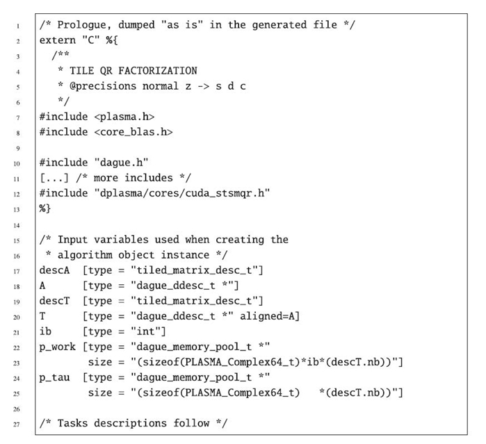
FIGURE 32.6. Samples from the JDF of the QR algorithm: prologue.

Then, the JDF file contains the description of all the task classes, usually generated automatically from the decorated sequential code. For each task class, the programmer needs to define (1) the data affinity of the tasks (: A.mat(k, n) in Fig. 32.3) and (2) user-provided bodies, which are, in the case of linear algebra, usually as simple as calling a BLAS or PLASMA kernel. Sometimes, algorithmic technicalities result in additional work for the programmer: Many kernels of the QR algorithm use a temporary scratchpad memory (the phony arguments in Figure 32.5). This memory is purely local to the kernel itself; hence, it does not need to appear in the dataflow. However, to preserve Fortran compatibility, scratchpad memory needs to be allocated outside the kernels themselves and passed as an argument. As a consequence, the bodies have to allocate and release these temporary arrays. We have designed a set of helper functions while designing DPLASMA, whose purpose is to ease the writing of linear algebra bodies; the code presented in Figure 32.7 illustrates how the programmer can push and pop scratchpad memory from a generic system call free memory pool. The variable name translation table, dumped automatically by the sequential code dependency extractor, helps the programmer navigate the generated dependencies and select the appropriate variable as a parameter of the actual computing kernel.

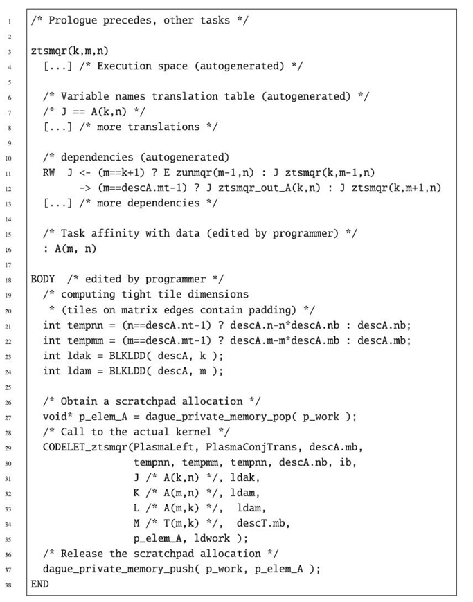
FIGURE 32.7. Samples from the JDF of the QR algorithm: task body.

32.5.2.1   Accelerator Port   The only action required from the linear algebra package to enable GPU acceleration is to provide the appropriate codelets in the body part of the JDF file. A codelet is a piece of code that encapsulates a variety of implementations of an operation for a variety of hardware. Just like CPU core kernels, GPU kernels are sequential and pure; hence, a codelet is an abstraction of a computing function suitable for a variety of processing units, either a single core or a single GPU stream (even though they can still contain some internal parallelism, such as vector single-instruction multiple-data [SIMD] instructions). Practically, that means that the application developer is in charge of providing multiple versions of the computing bodies. The relevant codelets, optimized for the current hardware, are loaded automatically during the algorithm initialization (one for the GPU hardware, one for the CPU cores, etc.). Today, the DAGUE runtime supports only CUDA and CPU codelets, but the infrastructure can easily accommodate other accelerator types (Intel Many Integrated Core [MIC or Xeon Phi], Open Computing Language [OpenCL], field-programmable gate arrays [FPGAs], Cell, etc.). If a task features multiple codelets, the runtime scheduler chooses dynamically (during the invocation of the automatically generated scheduling hook codeLET_kernelname) between all these versions in order to execute the operation on the most relevant hardware. Because multiple versions of the same codelet kernel can be in use at the same time, the workload of this type of operations, on different input data, can be distributed on both CPU cores and GPUs simultaneously.

In the case of the QR factorization, we selected to add a GPU version of the STSMQR kernel, which is the matrix‒matrix multiplication kernel used to update the remainder of the matrix, after a particular panel has been factorized (hence representing 80% or more of the overall compute time). We have extended a hand-made GPU kernel [34], originally obtained from MAGMA [12]. This kernel is provided in a separate source file and is developed separately as a regular CUDA function. Should future versions of CuBLAS enable running concurrent GPU kernels on several hardware streams, these vendor functions could be used directly.

32.5.2.2   Wrapper   As previously stated, scratchpad memory needs to be allocated outside of the bodies. Similarly, because we wanted the JDF format to be oblivious of the transport technology, data types, which are inherently dependent on the description used in the message-passing system, need to be declared outside the generated code. In order for the generated library to be more convenient to use for end users, we consider it good practice to provide a wrapper around the generated code that takes care of allocating and defining these required elements. In the case of linear algebra, we provide a variety of helper functions to allocate scratch-pads (line 9 in Fig. 32.8), and to create most useful data types (like triangular matrices) (lines 13 and 18 in the same figure), like band matrices and square or rectangular matrices. Again, the framework-provided tool can create all floating-point precisions from a single source.

32.5.2.3   Main Program   A skeleton program that initializes and schedules a QR factorization using the DAGUE framework is presented in Figure 32.9. Since DAGUE uses MPI as an underlaying communication mechanism, the test program is an MPI program. It thus needs to initialize and finalize MPI (lines 8 and 33) and the programmer is free to use any MPI functionality, around DAGUE calls (line 9, where arguments should also be parsed). A subset of the DAGUE calls is to be considered as a collective operation from an MPI perspective: All MPI processes must call them in the same order, with a communication scheme that allows these operations to match. These operations are the initialization function(dague_init), the progress function(dague_progress), and the finalization function(dague_fini). dague_init will create a specified number of threads on the local process, plus the communication thread. Threads are bound on separate cores when possible. Once the DAGUE system is initialized on all MPI processes, each must choose a local scheduler. DAGUE provides four scheduling heuristics, but the one preferred is the Local Hierarchical Scheduler, developed specifically for DAGUE on NUMA many-core heterogeneous machines. The function dague_set_scheduler of line 12 sets this scheduler.

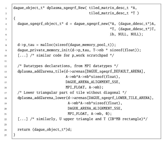
FIGURE 32.8. User‒provided wrapper around the DAGUE generated QR factorization function.

The next step consists of creating a data distribution descriptor. This code holds two data distribution descriptors: ddescA and ddescT. DAGUE provides three built-in data distributions for tiled matrices: an arbitrary index-based distribution, a symmetric 2-D block-cyclic distribution, and a 2-D block-cyclic distribution. In the case of QR, the latter is used to describe the input matrix A to be factorized and the workspace array T. Once the data distribution is created, the local memory to store this data should be allocated in the fields mat of the descriptor. To enableDAGUE to pin memory, and allow for direct DMA transfers (to and from the GPUs or some high-performance networks), the helper function dague_data_allocate of line 15 is used. The workspace array T should be described and allocated in a similar way on line 16.

Then, this test program uses DPLASMA functions to initialize the matrix A with random values (line 18), and the workspace array T with 0 (line 19). These functions are coded in DAGUE: They create a DAG representation of a map operation that will initialize each tile in parallel with the desired values, making the engine progress on these DAGs.

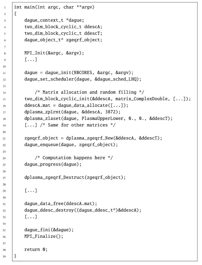
FIGURE 32.9. Skeleton of a DAGUE main program driving the QR factorization.

Once the data are initialized, a zgeqrf DAGUE object is created with the wrapper that was described above. This object holds the symbolic representation ofthe local DAG, initialized with the desired parameters and bound to the allocated and described data. It is (locally) enqueued in the DAGUE engine on line 22.

To compute the QR operation described by this object, all MPI processes call to dague_progress on line 24. This enables all threads created on line 8 to work on the QR operation enqueued before in collaboration with all the other MPI processes. This call returns when all enqueued objects are completed, thus, when the factorization is done. At this point, the zgeqrd DAGUE object is consumed and can be freed by the programmer at line 26. The result of the factorization should be used on line 28, before the data are freed (line 30), and the descriptors destroyed (line 31). Line 32 should hold a similar code to free the data and destroy the descriptor of T. Then, the DAGUE engine can release all resources (line 34) before MPI is finalized and the application terminates.

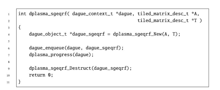
FIGURE 32.10. DPLASMA SPMD interface for the DAGUE generated QR factorization function.

32.5.2.4   SPMD Library Interface   It is possible for the library to encapsulate all dataflow-related calls inside a regular (ScaLAPACK like) interface function. This function creates an algorithm instance, enqueues it in the dataflow runtime, and enables progress (lines 6, 7, and 9 in Fig. 32.10). From the main program point of view, the code is similar to a SPMD call to a parallel BLAS function; the main program does not need to consider the fact that dataflow is used within the linear algebra library. While this approach can simplify the porting of legacy applications, it prevents the program from composing DAG-based algorithms. If the main program takes full control of the algorithm objects, it can enqueue multiple algorithms and then progress all of them simultaneously, enabling optimal overlap between separate algorithms (such as a factorization and the associated solve); if it simply calls the SPMD interface, it still benefits from complete parallelism within individual functions, but it falls back to a synchronous SPMD model between different algorithms.

32.5.3  Correctness and Performance Analysis Tools

The first correctness tool of the DAGUE framework sits within the code generator tool, which converts the JDF representation into C functions. A number of conditions on the dependencies and execution spaces are checked during this stage and can detect many instances of mismatching dependencies (where the input of task A comes from task B, but task B has no outputs to task A). Similarly, conditions that are not satisfiable according to the execution space raise warnings, as is the case for pure input data (operations that read the input matrix directly, not as an output of another task) that do not respect the task‒data affinity. These warnings help the programmer detect the most common errors when writing the JDF.

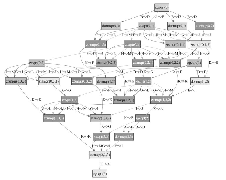
FIGURE 32.11. The runtime can output a graphical version of the DAG for validation purposes. In this example, the output shows the execution of the QR operation on a 4 × 4 tiled matrix, on two nodes with eight cores per node.

At runtime, algorithm programmers can generate the complete unrolled DAG for offline analysis purposes. The DAGUE engine can output a representation of the DAG, as it is executed, in the dot input format of the GraphViz graph plotting tool. The programmer can use the resulting graphic representation (see Fig. 32.11) to analyze which kernel ran on what resource, and which dependence released which tasks into their ready state. Using such information has proven critical when debugging the JDF representation (for an advanced user who wants to write his or her own JDF directly without using the DAGUE compiler), or to understand contentions and improve the data distribution and the priorities assigned to tasks.

The DAGUE framework also features performance analysis tools to help programmers fine-tune the performance of their application. At the heart of these tools, the profiling collection mechanism optionally records the duration of each individual task, communication, and scheduling decision. These measurements are saved in thread-specific memory, without any locking or other forms of atomic operations, and are then output at termination time in an XML file for offline analysis.

This XML file can then be converted by tools provided in the framework to portable trace formats (like open trace format [OTF] [35]), or simple spreadsheets, representing the start date and duration of each critical operation. Figure 32.12 presents two Gantt chart representations of the beginning of a QR DAGUE execution on a single node, eight cores using two different scheduling heuristics: the simple first in, first out (FIFO) scheduling and the scheduler of DAGUE (local hierarchical queues, described in Section 32.3.1). The ability of the local hierarchical queues scheduler to increase the data locality, allow for maximal parallelism, and avoid starvations is highlighted in these graphs. Potential starvations are easily spotted, as they appear as large stripes where multiple threads do not execute any kernel. Similar charts can be generated for distributed runs (not presented here), with a clear depiction of the underlying communications in the MPI thread, annotated by the data they carry and tasks they connect. Using these results, a programmer can assess the efficiency, on real runs, of the proposed data distribution, task affinity, and priority. Data distribution and task affinity will both influence the amount and duration of communications, as well as the amount of starvation, while priority will mostly influence the amount of starvation.

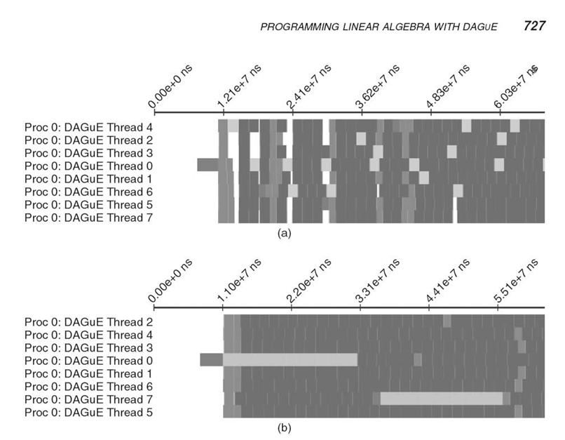
FIGURE 32.12. Gantt representation of a shared-memory run of the QR factorization on 8 threads.

In the case of the QR factorization, these profiling outputs have been used to evaluate the priority hints given to tasks, used by the scheduler when ordering tasks (refer to Section 32.3.1). The folklore knowledge about scheduling DAG of dense factorizations is that the priorities should always favor the tasks that are closer to the critical path. We have implemented such a strategy and discovered that it is easily outperformed by a completely dynamic scheduling that does not respect any priorities. There is indeed a fine balance between following the absolute priorities along the critical path, which enables maximum parallelism, and favoring cache reuse even if it progresses a branch that is far from the critical path. We have found a set of beneficial priority rules (which are symbolic expressions similar to the dependencies) that favor progressing iterations along the k direction first, but favor only a couple iterations of the critical path over update kernels.

32.6  PERFORMANCE EVALUATION

The performance of the DAGUE runtime has been extensively studied in related publications [4,34,36]. The goal here is to illustrate the performance results that can be achieved by the porting of linear algebra code to the DAGUE framework. Therefore, we present a summary of these results to demonstrate that the tool chain achieves its main goals of overall performance, performance portability, and capability to process different nontrivial algorithms.

The experiments we summarize here have been conducted on three different platforms. The Griffon platform is one of the clusters of Grid’5000 [37]. We used 81 dual socket Intel Xeon L5420 quad core processors at 2.5 GHz to gather 648 cores. Each node has 16 GB of memory and is interconnected to the others by a 20‒Gb Infiniband network. Linux 2.6.24 (Debian Sid) is deployed on these nodes. The Kraken system of the University of Tennessee and National Institute for Computational Science (NICS) is hosted at the Oak Ridge National Laboratory. It is a Cray XT5 with 8256 compute nodes connected on a 3-D torus with SeaStar. Each node has a dual six-core AMD Opteron cadenced at 2.6 GHz. We used up to 3072 cores in the experiments we present here. All nodes have 16 GB of memory and run the Cray Linux Environment (CLE) 2.2.

The benchmark consists of three popular dense matrix factorizations: Cholesky, LU, and QR. The Cholesky factorization solves the problem Ax = b, where A is symmetric and positive definite. It computes the real lower triangular matrix with positive diagonal elements L such that A = LL^T. The QR factorization has been presented in previous sections, to explain the functionality and behavior of DAGUE. It offers a numerically stable way of solving full rank underdetermined, overdeter-mined, and regular square linear systems of equations. It computes Q and R such that A = QR, Q is a real orthogonal matrix, and R is a real upper triangular matrix. The LU factorization with partial pivoting of a real matrix A has the form PA = LU, where L is a real unit lower triangular matrix, U is a real upper triangular matrix, and P is a permutation matrix.

All three of these operations are implemented in the ScaLAPACK numerical library [38]. In addition, some of these factorizations have more optimized versions; we used the state-of-the-art version for each of the existing factorizations to measure against. The Cholesky factorization has been implemented in a more optimized way in the DSBP software [16] using static scheduling of tasks and a specific, more efficient data distribution. The LU factorization with partial pivoting is also solved by the well-known high-performance LINPACK (HPL) benchmark [39], used to measure the performance of high-performance computers. We have distributed the initial data following a classical 2-D block-cyclic distribution used by ScaLAPACK and have used the DAGUE runtime engine to schedule the operations on the distributed data. The kernels consist of the BLAS operations referenced by the sequential codes, and their implementation was the most efficient, available on each of the machine.

Figure 32.13 presents the performance measured for DAGUE and ScaLAPACK, and when applicable, DSBP and HPL, as a function of the problem size. Six hundred forty-eight cores on 81 multicore nodes have been used for the distributed run, and the data were distributed according to a 9 × 9 2-D block-cyclic grid for DAGUE. A similar distribution was used for ScaLAPACK, and the other benchmarks when appropriate, and the block size was tuned to provide the best performance on each setup. As the figures illustrate, on all benchmarks, and for all problem sizes, the DAG E framework was able to outperform ScaLAPACK and to perform as well as the state-of-the-art, hand-tuned codes for specific problems. The DAGUE approach, that is, completely automatic conversion from sequential code to the corresponding parallel version, is able to outperform DSBP and compete favorably with the HPL implementation on this machine.

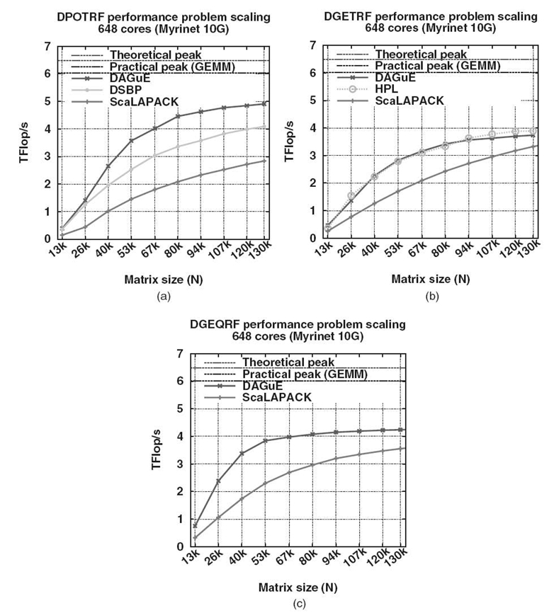
FIGURE 32.13. Performance comparison on the Griffon platform with 648 cores.

Figure 32.14a presents the performance of the DAGUE Cholesky algorithm on a GPU cluster, featuring 12 Fermi C2070 accelerators (one per node). Without GPU accelerators, the DAGUE runtime extracts the entire available performance; asymptotic performance matches the performance of the GEMM kernel on this processor, which is an upper bound to the effective peak performance. When using one GPU accelerator per node, the total efficiency reaches as much as 73% of the GEMM peak, which is a 54% efficiency of the theoretical peak (typical GPU efficiency is lower than CPU efficiency; the HPL benchmark on the TianHe‒1A GPU system reaches a similar 51% efficiency, which compares with 78% on the CPU‒based Kraken machine). Scalability is a concern with GPU accelerators as they provoke a massive imbalance between computing power and network capacity. Figure 32.14b presents the Cholesky factorization weak scalability (the number of nodes varies; problem size grows accordingly to keep memory load per node constant) on the GPU enabled machine. The figure outlines the perfect weak scalability up to 12 GPU nodes.

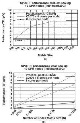
FIGURE 32.14. Performance of DAGUE Cholesky on the Dancer GPU accelerated cluster.

Last, Figure 32.15 compares the performance of the DAGUE implementation of these three operations with the libSCI implementation, specifically tuned by Cray for this machine. The value represented is the relative time overhead of DAGUE compared to libSCI for different matrix sizes and the number of nodes on the QR factorization (similar weak scaling as in the previous experiment, N = 454,000 on 3072 cores). On this machine, the DAGUE runtime can effectively use only 11 of 12 cores per node for compute tasks; due to kernel scheduler parameters (long, non-preemptive time quantum), the MPI thread must be exclusively pinned to a physical core to avoid massive and detrimental message jitter. Even considering that limitation, which is only technical and could be overcome by a native port of the runtime to the portal messaging library instead of MPI, the DAGUE implementation competes favorably with the extremely efficient libSCI QR factorization. The DAGUE approach demonstrates an excellent scalability, up to a massive number of nodes, thanks to the distributed evaluation of the DAG not requiring centralized control nor complete unrolling of the DAG on each node.

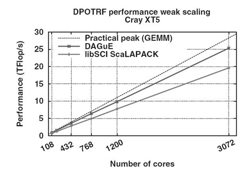
FIGURE 32.15. Scalability on the Kraken platform.

On different machines, the DAGUE compiler coupled with the DAGUE runtime significantly outperformed standard algorithms and competed closely, usually favorably, with state‒of‒the‒art optimized versions of similar algorithms, without any further tuning process involved when porting the code between radically different platform types. Another significant fact to be highlighted is the sizes of the problem where DAGUE achieves peak performance. In all graphs in Figure 32.13, one can notice that while ScaLAPACK asymptotically reaches peak performance, for some of the algorithms, DAGUE achieves the same level of performance on data four times smaller (in the case of Cholesky, ScaLAPACK achieves 3 Tflop/s on Griffon when N = 130,000, while DAGUE reaches the same level for N = 44,000).

32.7  CONCLUSION

Although hardware architectural paradigm shifts are threatening the scientific productivity of dense linear algebra codes, we have demonstrated that by slightly changing the execution paradigm and using a dataflow representation extracted from a decorated sequential code, dense matrix factorization can reach excellent performance. The DPLASMA package aims at providing the same functionalities as the ScaLAPACK legacy package, but using a more modern approach, based on tile algorithm and dataflow representation, that enables better cache reuse and asynchrony, which are paramount features to perform on multicore nodes. Furthermore, the DAG dataflow representation enables the algorithm to adapt easily to a variety of differing and heterogeneous hardware, without involving a major code refactoring for each target platform. We describe how the DPLASMA project uses the DAGUE framework to convert a decorated sequential code (which can be executed efficiently on multicore machines but not on distributed‒memory systems) into a concise DAG dataflow representation. This representation is then altered by the programmer to add data distribution and task affinity on distributed memory. The resulting intermediate format is then compiled into a series of runtime hooks incorporating a DAG scheduler that automatically orchestrates the resolution of remote dependencies, orchestrates the execution to favor cache locality and other scheduling heuristics, and accounts for the presence of heterogeneous resources such as GPU accelerators. This description gives insight to linear algebra programmers as to the methods, challenges, and solutions involved in porting their code to a dataflow representation. The performance analysis section demonstrates the vast superiority of the DAG‒based code over legacy programming paradigms on newer multicore hardware.

32.8  SUMMARY

The tumultuous changes occurring in the computer hardware space, such as flatlining of processor clock speeds after more than 15 years of exponential increases, mark the end of the era of routine and near‒automatic performance improvements that the research community had previously enjoyed [40]. Two main factors converged to force processor architects to turn to multicore and heterogeneous designs and, consequently, to bring an end to the “free ride.” First, system builders have encountered intractable physical barriers—too much heat, too much power consumption, and too much leaking voltage—to further increases in clock speeds. Second, physical limits on the number of pins and bandwidth on a single chip mean that the gap between processor performance and memory performance, which was already bad, has gotten increasingly worse. Consequently, the design trade‒offs made to address the previous two factors rendered commodity processors, absent any further augmentation, inadequate for the purposes of extreme‒scale systems for advanced applications. This daunting combination of obstacles forced the designers of new multicore and hybrid systems to explore architectures that software built on the old model are unable to effectively exploit without radical modification.

To develop software that will perform well on extreme‒scale systems with thousands of nodes and millions of cores, the list of major challenges that must now be confronted is intimidating:

• Automatic adaptation to the dramatic escalation in the costs of intrasystem communication between processors and/or levels of memory hierarchy
• Acclimatization to the increased hybridization of processor architectures (mixing CPUs, GPUs, etc.), in varying and unexpected design combinations
• Cooperating processes must be dynamically and unpredictably scheduled for asynchronous execution due to high levels of parallelism and more complex constraints.
• Software will not run at scale without much better resilience to faults and increased robustness.
• New levels of self‒adaptivity will be required to enable software to modulate process speed in order to satisfy limited energy budgets.

The software project presented above meets the aforementioned challenges and allows the users to run their computationally intensive codes at scale and to achieve a significant percentage of peak performance on the contemporary hardware systems that may soon break the barrier of 100 Pflop/s. This is achieved by finding and integrating solutions to problems in two critical areas: novel algorithm design as well as management of parallelism and hybridization.

REFERENCES

[1] P. Kogge, K. Bergman, S. Borkar, D. Campbell, W. Carlson, W. Dally, M. Denneau, P. Franzon, W. Harrod, K. Hill, J. Hiller, S. Karp, S. Keckler, D. Klein, R. Lucas, M. Richards, A. Scarpelli, S. Scott, A. Snavely, T. Sterling, R.S. Williams, and K. Yelick, “Exascalecomputing study: Technology challenges in achieving exascale systems,” Technical Report TR-2008-13, Department of Computer Science and Engineering, University of Notre Dame, September 28 2008.

[2] National Research Council Committee on the Potential Impact of High‒End Computing on Illustrative Fields of Science and Engineering, The Potential Impact of High‒End Capability Computing on Four Illustrative Fields of Science and Engineering. Washington, DC: National Academies Press, 2008.

[3] University of Tennessee, PLASMA Users’ Guide, Parallel Linear Algebra Software for Multicore Architectures, Version 2.2, November 2009.

[4] G. Bosilca, A. Bouteiller, A. Danalis, T. Herault, P. Lemarinier, and J.J. Dongarra, “DAGUE: A generic distributed DAG engine for high performance computing,” Parallel Computing, 38: 37‒51, 2011.

[5] E.G. Coffman, Jr. and P.J. Denning, Operating Systems Theory. Upper Saddle River, NJ: Prentice Hall Professional Technical Reference. 1973.

[6] A.J. Bernstein, “Analysis of programs for parallel processing,” IEEE Transactions on Electronic Computers, EC-15: 757‒763, 1966.

[7] J.A. Sharp ed., Data Flow Computing: Theory and Practice. Norwood, NJ: Ablex Publishing Corp., 1992.

[8] J. Yu and R. Buyya, “A taxonomy of workflow management systems for grid computing,” Technical Report, Journal of Grid Computing, 3: 171‒200, 2005.

[9] O. Delannoy, N. Emad, and S. Petiton, “Workflow global computing with YML,” 7th IEEE/ACM International Conference on Grid Computing, September 2006.

[10] A. Buttari, J.J. Dongarra, J. Kurzak, J. Langou, P. Luszczek, and S. Tomov, “The impact of multicore on math software,” in Applied Parallel Computing, State of the Art in Scientific Computing, 8th International Workshop, PARA, Vol. 4699 of Lecture Notes in Computer Science, pp. 1‒10, Springer, 2006.

[11] E. Chan, F.G. Van Zee, P. Bientinesi, E.S. Quintana‒Ortĺ, G. Quintana‒Ortĺ, and R.van de Geijn, “Supermatrix: A multithreaded runtime scheduling system for algorithms‒by -blocks,” in PPoPP’08: Proceedings of the 13th ACM SIGPLAN Symposium on Principles and Practice of Parallel Programming, pp. 123‒132, ACM, 2008.

[12] E. Agullo, J. Demmel, J.J. Dongarra, B. Hadri, J. Kurzak, J. Langou, H. Ltaief, P. Luszczek, and S. Tomov, “Numerical linear algebra on emerging architectures: The PLASMA and MAGMA projects,” Journal of Physics: Conference Series, 180: 12‒37, 2009.

[13] R. Dolbeau, S. Bihan, and F. Bodin, “HMPP: A hybrid multi‒core parallel programming environment,” in Workshop on General Purpose Processing on Graphics Processing Units (GPGPU 2007), 2007.

[14] C. Augonnet, S. Thibault, R. Namyst, and P.‒A. Wacrenier, “StarPU: A unified platform for task scheduling on heterogeneous multicore architectures,” Concurrency and Computation: Practice and Experience, 23(2): 187‒198, 2011.

[15] P. Husbands and K.A. Yelick, “Multi‒threading and one‒sided communication in parallel LU factorization,” in Proceedings of the ACM/IEEE Conference on High Performance Networking and Computing, SC 2007 November 10‒16, 2007 (B. Verastegui, ed.), Reno, NV: ACM Press, 2007.

[16]F.G. Gustavson, L. Karlsson, and B. Kågström, “Distributed SBP Cholesky factorization algorithms with near‒optimal scheduling,” ACM Transactions on Mathematical Software, 36(2): 1‒25, 2009.

[17] J. Perez, R. Badia, and J. Labarta, “A dependency‒aware task‒based programming environment for multi‒core architectures,” 2008 IEEE International Conference on Cluster Computing, pp. 142‒151, October 1‒29, 2008.

[18] F. Song, A. YarKhan, and J.J. Dongarra, “Dynamic task scheduling for linear algebra algorithms on distributed‒memory multicore systems,” in SC’09: Proceedings of the Conference on High Performance Computing Networking, Storage and Analysis, pp. 1‒11, New York: ACM, 2009.

[19] M. Cosnard and E. Jeannot, “Automatic parallelization techniques based on compact DAG extraction and symbolic scheduling,” Parallel Processing Letters, 11: 151‒168, 2001.

[20] M. Cosnard, E. Jeannot, and T. Yang, “Compact dag representation and its symbolic scheduling,” Journal of Parallel and Distributed Computing, 64: 921‒935, 2004.

[21] E. Jeannot, “Automatic multithreaded parallel program generation for message passing multiprocessors using parameterized task graphs,” International Conference “Parallel Computing 2001” (ParCo2001), September 2001.

[22] A. Haidar, H. Ltaief, A. YarKhan, and J.J. Dongarra, “Analysis of dynamically scheduled tile algorithms for dense linear algebra on multicore architectures,” Concurrency and Computation: Practice and Experience, 24: 305‒321, 2011.

[23] AMD, “Amd64 architecture programmer’s manual volume 2: System programming,” Technical Report, AMD64 Technology, 2011.

[24] W. Pugh, “The omega test: A fast and practical integer programming algorithm for depend ence analysis,” in Supercomputing ’91: Proceedings of the 1991 ACM/IEEE Conference on Supercomputing, pp. 4‒13, New York, 1991.

[25] R. Harrington, “Origin and development of the method of moments for field computation,” IEEE Antennas and Propagation Magazine, 32: 31‒35, 1990.

[26] J.J.H. Wang, Generalized Moment Methods in Electromagnetics. New York: John Wiley & Sons, 1991.

[27] J.L. Hess, “Panel methods in computational fluid dynamics,” Annual Review of Fluid Mechanics, 22: 255‒274, 1990.

[28] L. Hess and M.O. Smith, “Calculation of potential flows about arbitrary bodies,” in Progress in Aeronautical Sciences (D. Kuchemann, ed.), Vol. 8. Pergamon Press, 1967.

[29] A. Edelman, “Large dense numerical linear algebra in 1993: The parallel computing influence,” International Journal of High Performance Computing Applications, 7(2): 113‒128, 1993.

[30] R.F. Barrett, T.H.F. Chan, E.F. D’Azevedo, E.F. Jaeger, K. Wong, and R.Y. Wong, “Complex version of high performance computing LINPACK benchmark (HPL),” Concurrency and Computation: Practice and Experience, 22(5): 573‒587, 2010.

[31] G.W. Stewart, “The decompositional approach to matrix computation,” Computing in Science & Engineering, 2: 50‒59, 2000.

[32] A. Buttari, J. Langou, J. Kurzak, and J.J. Dongarra, “Parallel tiled QR factorization for multicore architectures,” Concurrency and Computation: Practice and Experience, 20(13): 1573‒1590, 2008.

[33] R. Schreiber and C. van Loan, “A storage‒efficient WY representation for products of Householder transformations,” SIAM Journal on Scientific and Statistical Computing, 10: 53‒57, 1991.

[34] G. Bosilca, A. Bouteiller, T. Herault, P. Lemarinier, N. Saengpatsa, S. Tomov, and J.J. Dongarra, “Performance portability of a GPU enabled factorization with the DAGUE framework,” in Proceedings of the IEEE Cluster 2011 Conference (PPAC Workshop), pp. 395‒402, IEEE, September 2011.

[35] A.D. Malony and W.E. Nagel, “The open trace format (OTF) and open tracing for HPC,” Proceedings of the 2006 ACM/IEEE Conference on Supercomputing, SC’06, New York: ACM, 2006.

[36] G. Bosilca, A. Bouteiller, A. Danalis, M. Faverge, A. Haidar, T. Herault, J. Kurzak, J. Langou, P. Lemarinier, H. Ltaief, P. Luszczek, A. YarKhan, and J.J. Dongarra, “Flexible development of dense linear algebra algorithms on massively parallel architectures with DPLASMA,” in IEEE International Symposium on Parallel and Distributed Processing, 12th IEEE International Workshop on Parallel and Distributed Scientific and Engineering Computing (PDSEC‒11), pp. 1432‒1441, May 2011, Anchorage, AK.

[37] R. Bolze, F. Cappello, E. Caron, M. Daydé, F. Desprez, E. Jeannot, Y. Jégou, S. Lanteri, J. Leduc, N. Melab, G. Mornet, R. Namyst, P. Primet, B. Quetier, O. Richard, E.‒G. Talbi, and I. Touche, “Grid’5000: A large scale and highly reconfigurable experimental grid testbed,” International Journal of High Performance Computing Applications, 20(4): 481‒494, 2006.

[38] L.S. Blackford, J. Choi, A. Cleary, E. D’Azevedo, J. Demmel, I. Dhillon, J.J. Dongarra, S. Hammarling, G. Henry, A. Petitet, K. Stanley, D. Walker, and R.C. Whaley, ScaLAPACK Users’ Guide. Philadelphia, PA: Society for Industrial and Applied Mathematics, 1997.

[39] J.J. Dongarra, P. Luszczek, and A. Petitet, “The LINPACK benchmark: Past, present and future,” Concurrency and Computation: Practice and Experience, 15(9): 803‒820, 2003.

[40] H. Sutter, “The free lunch is over: A fundamental turn toward concurrency in software,” Dr. Dobb’s Journal, 30(3), 2005.

 

¹For this depiction, A.nt-2 was arbitrarily chosen to be smaller than A.mt-1, but in the general case, they can have any relation between them.

²The actual term used in PLASMA is “QUARK_Insert_Task,” but we abbreviate it here to “Task” for readability reasons.