
Audio power analysis
This article extended the idea of power-partition diagrams to include real waveforms of real music, and therefore required rather a lot of tedious measurement to acquire the probability density data. One of the surprises was that very different musical genres had very similar statistics. It was however reassuring to discover that the demands made on an amplifier by a sinewave were greater than those for music, but not wildly out of line. In other words, sinewave testing builds in a safety margin – if it works on sinewaves it will certainly survive music. Sinewave testing has received a lot of unkind criticism over recent years, but it continues unabated for the simple reason that it works.
Writing this put me off designing Class-A amplifiers for a long time. A branch of technology with a practical energy efficiency of less than 1% needs a good justification for its existence, and the distortion from a Blameless Class-B amplifier is so low that the extra linearity of Class-A amplifiers is no longer the forceful argument it was.
My last chapter showed how the power consumed by amplifiers of various classes was partitioned between internal dissipation and the power delivered to the load.1 This was determined for the usual sinewave case.
The snag with this approach is that a sinewave does not remotely resemble real speech or music in its characteristics. In many ways it is almost as far from it as you could get.
In particular, it is well-known that music has a large peak-to-mean ratio, or PMR, though the actual value of this ratio in decibels is a vague quantity. Signal statistics for music appear to be in surprisingly short supply.
Very roughly, general-purpose rock music has a PMR of 10 dB to 30 dB, while classical orchestral material – which makes very little use of fuzz boxes and the like – is 20 to 30 dB. The muzak you endure in lifts is limited in PMR to 3 to 10 dB, while compressed bass material in live PA systems is similar.
It is clear that the power dissipation in PA bass amplifiers is going to be radically different from that in hi-fi amplifiers reproducing orchestral material at the same peak level. The PMR of a sinewave if 4.0 dB, so results from this are only relevant to lifts.
Recognising that music actually has a peak-to-mean ratio is a start, but it is actually not much help as it reduces the statistics of signal levels to a single number. This does not give enough information for the estimation of power dissipation with real signals.
To calculate the actual power dissipations, two things are needed; a plot of the instantaneous power dissipations against level, and a description of how much time the signal spends at each level. The latter is formally called the ‘probability density function’, or PDF, of the signal; more on this later.
The instantaneous power partition diagram, or IPPD, is obtained by running the output stage simulation with a sawtooth input and no per-cycle averaging. Instantaneous power dissipation can therefore be read out for any input voltage fraction simply by running the cursor up the sawtooth.
Figure 1 is the instantaneous power partition diagram for the Class-B complementary-feedback pair case, where the quiescent current is very small. This looks very much like the averaged-sinewave power partition diagram in reference,1 but with the device dissipation maximum at 50% voltage rather than 64% for the sinewave case.
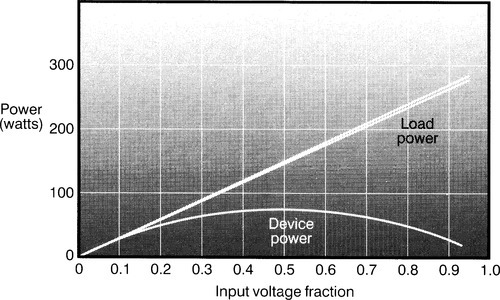
The instantaneous powers are much higher, as they are not averaged over a cycle. There is only one device-power area at the bottom as only one device conducts at a time. Output device dissipation at the moment when the signal is halfway between rail and ground, input fraction 50% – is 76 W, and the power in the load is 75 W. This total to 151 W, on the lower of the two straight lines, while the power drawn from the supply is shown as 153 W by the upper straight line. The 2 W difference represents losses in the driver transistors and the output emitter resistors.
All the IPPDs for various output stages look very similar in shape to the averaged-sine PPDs in Ref. 1, but the peak values on the Y-axis are higher. The IPPD can be combined with any PDF to give a much more realistic picture of how power dissipation changes as the level of a given type of signal is altered.
The probability density function
The most difficult part of the process above is obtaining the probability density function. For repetitive waveforms the PDF can be calculated,2 but music and speech need a statistical approach. It is often assumed that musical levels have a Gaussian (normal) probability distribution, as the sum of many random variables.
Positive statements on this are however hard to find. Benjamin3 says, ‘music can be represented accurately as a Gaussian distribution’ while Raad4 states, ‘music and mixed sounds typically have Gaussian PDFs’. It appears likely this assumption is true for multi-part music which can be regarded as a summation of many random processes; whatever the PDF of each component, the result is always Gaussian as indicated by the Central Limit Theorem.
If the distribution is Gaussian, its mean is clearly zero, as there is no DC component, which leaves the variance – i.e. width of the bell-curve – as the only parameter left to determine. The Gaussian distribution tails off to infinity, implying that enormous levels can occur, though very rarely.
In reality the headroom is fixed. I have dealt with this by setting variance so the maximum value, 0 dB. occurs 1% of the time. This is realistic as music very often requires judicious limiting of occasional peaks to optimise the dynamic range.
The PDF presents some conceptual difficulties, as it shows a density rather than a probability. If a signal level ranges between 0 and 100%, then clearly it might be expected to spend some of its time around 50%.
However, the probability that it will be at exactly 50.000% is zero, because a single level value has zero extent. Hence the PDF at x is the probability that the signal variable is in the interval (x, x + dx), where dx is the usual calculus infinitesimal.
The cumulative distribution function
If the probability that the instantaneous voltage will be above – not at – a given level is plotted against that level, a cumulative distribution function, or CDF, results. This is important as it is easier to measure than the PDF.
If the variable is x, then the PDF is often called P(x) and the CDF called F(x). These are related by:
![]()
or,
![]()
where a is a dummy variable needed to perform the integration. The integration starts at zero in this case because signal levels below zero do not occur.
Generating a CDF by integrating a given PDF is straightforward, but going the other way – determining the PDF from the CDF – can be troublesome as the differentiation accentuates noise on the data.
Some probability density functions
Figure 2 shows the calculated PDF of a sinewave. As with every PDF, the area under the curve is one, because the signal must be at some level all of the time.

However, the function blows up – i.e. heads off to infinity – at each end because the peaks of the wave are ‘flat’, and so the signal dwells there for infinitely longer than on the slopes where things are changing. These ‘flat’ bits are infinitely small in time extent though, and so the area under the curve is still unity. This shows you why PDFs are not always the easiest things to handle.
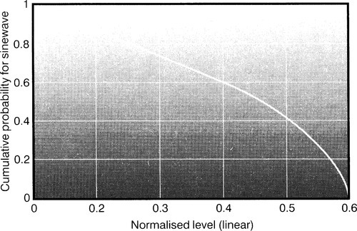
The CDF for a sinewave is shown in Figure 3; the probability of exceeding the level on the axis falls slowly at first, but then accelerates to zero as the rounded peaks are reached.
Measuring probability density functions
But is all music Gaussian? I was not satisfied that this had been conclusively established from just two brief references.
I decided it was essential to make some attempt to determine musical PDFs. In essence this is simple. The first thing to decide is the length of time over which to examine the signal. For most contemporary music the obvious answer is ‘one track’, a complete composition lasting typically between three and eight minutes.
Very simple circuitry can be used to determine a CDF, and hence the PDF, though the process is protracted. A variable-threshold comparator is driven by the signal to be measured, and its output applied to a long-period averaging time-constant. Figure 4.
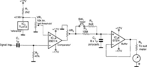
A comparator, IC1a, rather than an op-amp, is used to avoid inaccuracies due to slew-rate limiting. Reference IC2 is an inexpensive 2.56 V bandgap type, while VR1 sets the comparator threshold. When the signal level is below this threshold, the comparator open-collector output is off, and the voltage seen by the averaging network is zero.
When the signal exceeds threshold, the comparator output is pulled low, so this point carries an irregular rectangular waveform while signal is applied. The average value of this is derived by R3 and C2, buffered by IC3a, and drives a moving-coil meter through a suitable resistance R5.
Switch SW1 and R4 enable a quick reset when no signal is present. A moving-coil meter allows much easier reading of a changing signal, though not to any great accuracy.
Potentiometer VR2 sets the scale so that the meter deflects to full scale for a 100% reading. This is done with no input, so it is essential to check that the circuit offsets have put the comparator in the right state – i.e. output low; if not the inverting input will need to be pulled fractionally negative by a high-value biasing network.
The circuit only measures one polarity of the waveform, in this case the positive half, so signal symmetry is assumed. This is safe unless you plan to do a lot of work with solo instruments or single a cappella voices; the human vocal waveform is notably asymmetrical.
This minimal system is simple, but it only yields one data point at a time. Set the threshold level to say 50%, play the track – I’d pick a short one – and as it finishes the reading on the meter shows the percentage of time the signal exceeded the preset level.
Since twenty data points are required for a good graph, this gets pretty tedious. The four comparators of IC1 could give four points, if the timeconstant section was also quadrupled, and some means of freezing the output voltages provided.
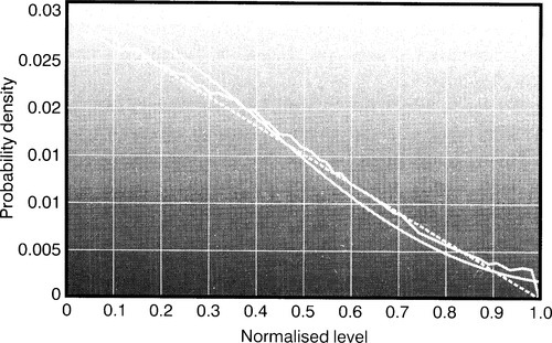
The CDF thus obtained for Alannah Myles’ ‘Black Velvet’ is Figure 5, and the PDF derived from it is Figure 6. It comes complete with some rather implausible ups and downs produced by differentiating data that is accurate to ± 1% at best.


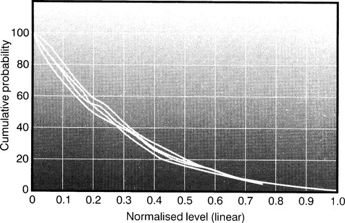
I measured several rock tracks, and also short classical works by Albinoni and Bach. The results are surprisingly similar; see the composite CDF in Figure 7. This is good news because we can use a single PDF to evaluate amplifiers faced with varying musical styles. However, I decided the method needed a reality check, by deriving the PDF in a completely different way.
Probability density functions via DSP
A digital processor offers the possibility of determining as many data points as you want on one playing of the music specimen. In this case a very simple 56001 program sorts the audio samples into 65 amplitude bins.
The result for 30 s of disco music is Figure 8, which is somewhere between triangular and Gaussian, if the latter has appropriate variance. The important point is that the difference between them is very small, and either can be used. The triangular PDF simplifies the mathematics, but if like me you use Mathcad to do the work, it is easy to plug in whatever distribution seems appropriate.
Deriving actual power
Having found the PDF, it is combined with the power partition diagram. In this case the IPPD is divided into twenty steps of voltage fraction, and each one multiplied by the probability the signal is in that region.
The summation of these products yields a single number – the average power dissipation in watts for a real signal that just reaches clipping for 1% of the time. An obvious extension of the idea is to plot the average power derived as above, against signal level on the X-axis. This gives an immediate insight into how amplifer power varies as the general signal level is reduced, as by turning down the volume control.
Figure 9 shows how level changes affect the PDF. Line 1 is maximum volume, just reaching full volume at the right. Line 2 is half volume, − 6 dB, and so hits the X-axis at 0.5; it is above Line 1 to the left as the probability of lower levels must be higher to maintain unity area under it.

This process continues as volume is reduced, until at zero volume the zero-level probability is 1 and all other levels have zero probability. Having generated twenty PDF functions, the powers that result for each one are plotted with the volume setting – not the output fraction – as the X-axis. The results for some common amplifer classes are as follows.
Class-B
The instantaneous power plot for Class-B complementary feedback pair combined with a triangular PDF of Figure 10 illustrates how the load and device power varies with volume setting. A signal with triangular PDF spends most of its time at low values, below 0.5 output fraction, and so there is no longer a dissipation maximum around half output. Device dissipation at bottom increases monotonically with volume. Load power increases with a square-law, which is a reassuring check on all these calculations.

Figure 11 is Figure 10 replotted with a logarithmic X-axis, which is more applicable to human hearing. Domestic amplifiers are rarely operated on the edge of clipping; a realistic operating point is more like − 15 or − 10 dB. The plot reveals that here the efficiency is low, with much more power dissipated in the devices than reaches the load.

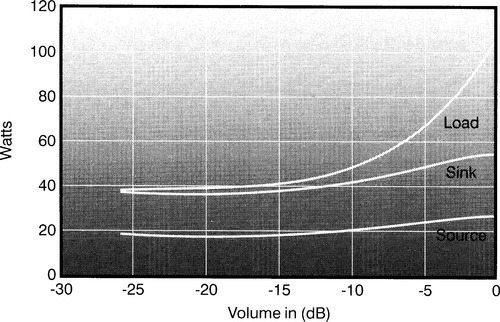
Class-AB
A decibel plot for Class-AB, biased so Class-A operation is maintained up to 5 W r.m.s. output is shown in Figure 12. Quiescent current is now 370 mA, so there is greater quiescent dissipation at zero volume. There is also substantial conduction overlap, and so sink and source would be different if the plot only considered voltage excursions in one direction away from 0 V. When positive and negative half-cycles are averaged, symmetry is achieved. The total device dissipation is unchanged but the boundary between the source and sink areas is half way, as in Figure 12.
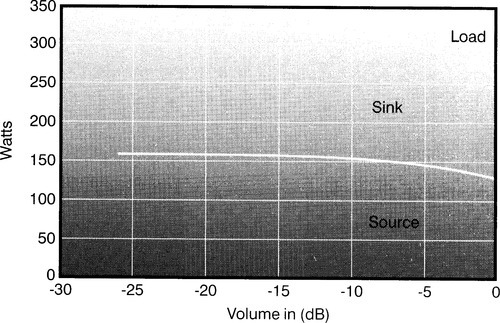
Class-A push-pull
I have stuck with the same ± 50 V rails for ease of comparison, and this yields a very powerful Class-A amplifier. The power drawn from the load is constant, and as output increases dissipation transfers from the output devices to the load, giving minimum amplifier heating at maximum output.
The result for sinewave drive is bad enough,1 but Figure 13 reveals that with real signals, almost all the energy supplied is wasted internally – even at maximum volume. Class-A has always been stigmatised as inefficient; this shows that under realistic conditions it is hopelessly inefficient, so much so that it grates on my sense of engineering aesthetics. At typical listening volumes of − 15 dB the efficiency barely reaches 1%.
Class-G
This class of amplifiers was introduced by Hitachi in 1976 to reduce amplifier power dissipation by exploiting the high peak-mean ratio of music.5 Class-G made little headway in the hi-fi market as the power saving does not outweigh the increased circuit complexity, but the rise of five-channel home theatre applications has caused a revival of interest in improved amplifier efficiency.
I recently explained Class-G in Ref. 6. At low outputs, power is drawn from low-voltage rails; for the relatively infrequent excursions into high power, higher rails are switched in.
In Figure 14 the lower rails are ± 15 V, 30% of the higher ± 50 V rails; I call this Class-G-30%. The lower area is the power in the inner devices – i.e. those in all the time. The larger area just above is that in the outer devices, i.e. those only activated when running from the higher rails. This is zero below the rail-switching threshold at a volume of 0.2.

Total device dissipation is reduced from 48 W in Class-B to 40 W, which is not a good return for twice as many power transistors. This is because the lower rail voltage is poorly chosen for signals with a triangular PDF.
If the low rails are increased to ± 30 V this become Class-G-60% as in Figure 15. Here the low-dissipation region now extends up to a voltage fraction of 0.5, but inner device dissipation is higher due to the increased lower rail voltages.

The overall result is that total device power is reduced from 48 W in Class-B to 34 W, which is a definite improvement. I am not suggesting that 60% is the optimum lower-rail voltage. The efficiency of Class-G amplifiers depends very much on signal statistics.
Reactive loads
The disadvantage of using instantaneous power is that it ignores signal and circuit history, and so cannot give meaningful information with reactive loads. The peak dissipations that these give rise to with real signals are difficult to simulate; it would be necessary to drive the circuit with stored music signals for many cycles; and that would only cover a few seconds of a CD or concert. The anomalous speaker currents examined in Ref. 7 show how significant history effects can be with some waveforms.
In summary
Tables 1 and 2 summarise how a triangular-PDF signal – rather than a sinewave – reduces average power dissipation, and the power drawn from the supply.
Table 1
Device dissipation, worst-case volume
| Sinewave (W) | PDF (W) | Factor | |
| Class-B CFP | 64 | 48 | 0.75 |
| Class-AB | 64 | 55 | 0.78 |
| Class-A, push-pull | 324 | 324 | – |
| Class-G-30% | 43 | 40 | 0.93 |
| Class-G-60% | 56 | 34 | 0.61 |
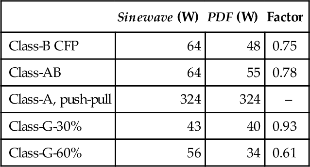
Table 2
Power drawn, worst-case. Always maximum output
| Sinewave (W) | PDF (W) | Factor | |
| Class-B CFP | 186 | 97 | 0.52 |
| Class-AB | 188 | 105 | 0.58 |
| Class-A, push-pull | 324 | 324 | – |
| Class-G-30% | 177 | 93 | 0.52 |
| Class-G-60% | 169 | 81 | 0.48 |

These economies are significant; the power amplifier market is highly competitive, and it is essential to exploit the cost savings in heat-sinks and ower-supply components made possible by designing for real signals rather than sinewaves.
In particular, Class-G shows valuable economies in device dissipation and ower-supply capacity, though to reduce dissipation, the lower supply voltage must be carefully chosen. This approach is unlikely to reduce the number of power devices required as real signals give no corresponding reduction in peak device power or peak device current.