Chapter 18
Signal-Present Indication
Some amplifiers and the more sophisticated mixers are fitted with a ‘signal-present’ indicator that illuminates to give reassurance that a channel is receiving a signal and doing something with it. The level at which it triggers must be well above the noise floor, but also well below the peak indication or clipping levels. Signal-present indicators are usually provided for each channel, and are commonly set up to illuminate when the channel output level exceeds a threshold 20 dB below the nominal signal level.
A vital design consideration is that since it may be active most of the time, the operation of the signal-present detector must not introduce distortion into the signal being monitored; this could easily occur by electrostatic coupling or imperfect grounding if there is a comparator switching on and off at signal frequency. A typical circuit would comprise just the bottom step of that of the LED bar-graph meter shown in Figure 18.4 below.

Figure 18.4: LED bar-graph meter circuit with selectable peak/average response
Peak Indication
A mixer has a relatively complex signal path, and the main metering is normally connected only to the group outputs. The mix metering can be used to measure the level in other parts of the signal path by use of the PFL system (see Chapter 17) if fitted, but this can only monitor one channel at a time. It is therefore usual to guard against clipping by fitting peak level indication to every channel of all but the simplest consoles, and sometimes to effect-return modules also.
The peak indicator is driven by fast-attack, slow-decay circuitry so that even brief peak excursions give a positive display. It is important that the circuitry should be bipolar, i.e. it will react to both positive and negative peaks. The peak values of a waveform can show asymmetry up to 8 dB or more, being greatest for unaccompanied voice or a single instrument, and this is of course very often exactly what goes through a mixer channel. This level of uncertainty in peak detection is not a good thing, so only the simplest implementations use unipolar peak detection. Composite waveforms, produced by mixing several voices or instruments together, do not usually show significant asymmetries in peak level.
Figure 18.1 shows a simple unipolar Peak LED driving circuit. This only responds to positive peaks, but it does have the advantage of using but two transistors and is very simple and cheap to implement. When a sufficient signal level is applied to C1, Q1 is turned on via the divider R1, R2; this turns off Q2, which is normally held on by R4, and Q2 then ceases to shunt current away from peak LED D1. C2 acts as a Miller integrator to stretch the peak hold time; when Q1 turns off again, R4 must charge C2 before Q2 can turn on again. Note that this circuit is integrated into the Channel On LED supply, with R5 setting the current through the two LEDs; the Channel On LED is illuminated by removing the short placed across it by SW1. R5 is of high enough value, because it is connected between the two supply rails, for there to be no significant variation in the brightness of one LED when the other turns off. If for some reason this was a critical issue, R5 could be replaced by a floating constant-current source. Other LEDs switched in the same way can be included in series with the Channel On LED.

Figure 18.1: A simple unipolar peak detector, including powering for the Channel On LED
This peak detect circuit has a non-linear input impedance and must only be driven from a low-impedance point, preferably direct from the output of an op-amp. The Peak LED illuminates at an input of 6.6 Vpeak, which corresponds to 4.7 Vrms (for a sine wave) and +16 dBu. For typical op-amp circuitry running off the usual supply rails this corresponds to having only 3 or 4 dB of headroom left. The detect threshold can be altered by changing the values of the divider R1, R2.
Distributed Peak Detection
When an audio signal path consists of a series of circuit blocks, each of which may give either gain or attenuation – and the classical example is a mixer channel with multiple EQ stages and a fader and postfade amplifier – it is something of a challenge to make sure that excessive levels do not occur anywhere along the chain. Simply monitoring the level at the end of the chain is no use because a circuit block that gives gain, leading to clipping, may be followed by one that attenuates the clipped signal back to a lower level that does not trip a final peak-detect circuit. The only way to be absolutely sure that no clipping is happening anywhere along the path is to implement bipolar peak detection at the output of every op-amp stage. This is, however, normally regarded as a bit excessive, and the usual practice in high-end equipment is to just monitor the output of each circuit block, even though each such block (for example, a band of parametric EQ) may actually contain several op-amps. It could be argued that a well-designed circuit block should not clip anywhere except at its output, no matter what the control setting, but this is not always possible to arrange.
A multi-point or distributed peak detection circuit that I have made extensive use of is shown in Figure 18.2. It can detect when either a positive or negative threshold is exceeded, at any number of points desired; to add another stage to its responsibilities you need only add another pair of diodes, so it is very economical. However, if one peak detector monitors too many points in the signal path, it can be hard to determine which of them is causing the problem. In most applications I have used the circuit to keep an eye on the output of the microphone preamplifier, the output of the EQ section, and the output of the fader postamplifier. This means that the location of the clipping can be pinpointed quite easily. If you pull down the fader to 0 dB or below and the Peak LED goes out, the problem was at the postfade amplifier. If that doesn’t do the trick, switch out the EQ; this assumes of course that the EQ in/out switch removes the signal feed to the unused EQ section. I always arrange matters so if possible, as removing the EQ signal reduces power consumption and minimizes the possibility of crosstalk. If that is not the case then you will have to back off any controls with significant boost and see if that works. Should the Peak indication persist, it must be coming from the output of the microphone preamplifier, and you will need to reduce the input gain.

Figure 18.2: A multi-point bipolar peak detector, monitoring three circuit blocks
The operation is as follows. Because R5 is greater than R1, normally the non-inverting input of the op-amp is held below the inverting input and the op-amp output is low. If any of the inputs to the peak system exceed the positive threshold set at the junction of R4, R3, one of D1, D3, D5 conducts and pulls up the non-inverting input, causing the output to go high. Similarly, if any of the inputs to the peak system exceed the negative threshold set at the junction of R2, R6, one of D2, D4, D6 conducts and pulls down the inverting input, once more causing the op-amp output to go high. When this occurs C1 is rapidly charged via D7. The output-current limiting of the op-amp discriminates against very narrow noise pulses. When C1 charges Q1 turns on, and illuminates D8 with a current set by the value of R7. R8 ensures that the LED stays off when U4 output is low, as it does not get close enough to the negative supply rail for Q1 to be completely turned off.
Each input to this circuit has a non-linear input impedance, and so for this system to work without introducing distortion into the signal path, it is essential that the diodes D1–D6 are driven directly from the output of an op-amp or an equivalently low impedance. Do not try to drive them through a coupling capacitor as asymmetrical conduction of the diodes can create unwanted DC shifts on the capacitor.
The peak-detect op-amp U4 must be an FET-input type to avoid errors due to bias currents flowing in the relatively high-value resistors R1–R6, and a cheap TL072 works very nicely here; in fact the resistor values could probably be raised significantly without any problems.
As with other non-linear circuits in this book, everything operates between the two supply rails so unwanted currents cannot find their way into the ground system.
Combined LED Indicators
For many years there has been a tendency towards very crowded channel front panels, driven by a need to keep the overall size of a complex console within reasonable limits. One apparently ingenious way to gain a few more square millimeters of panel space is to combine the signal-present and peak indicators into one by using a bicolor LED. Green shows signal present and red indicates peak. One might even consider using orange (both LED colors on) for an intermediate level indication.
Unfortunately, such indicators are hard to read, even with normal color vision. If you have red– green color-blindness, the most common kind (6% of males, 0.4% of females), they are useless. Combining indicators like this is not really a good idea.
VU Meters
VU meters are a relatively slow-response method of indicating an audio level in ‘Volume Units’. The standard VU meter was originally developed in 1939 by Bell Labs and the USA broadcasters NBC and CBS. The meter response is intentionally a ‘slow’ measurement that is intended to average out short peaks and give an estimate of perceived loudness. This worked adequately when it was used for monitoring the levels going to an analog tape machine, as the overload characteristic of magnetic tape is one of soft compression and the occasional squashing of short transient peaks is hard to detect aurally. Digital recorders overload in a much more abrupt and intrusive manner, making even brief overloads unpleasant, and the use of VU meters in professional audio has been in steady decline for many years.
The specifications, particularly of the dynamics, of a standard VU meter are closely defined in the documents British Standard BS 6840, ANSI C16.5-1942, and IEC 60268-17, but there are many cheap meters out there with ‘VU’ written on them that make no attempt to conform with these documents. The usual VU scale runs from −20 to +3, with the levels above zero being red; 1 VU is the same change in level as 1 dB. The rise and fall times of the meter are both 300 ms, so if a sine wave of amplitude 0 VU is applied suddenly, the needle will take 300 ms to swing over to 0 VU on the scale. A proper VU meter uses full-wave rectification so asymmetrical waveforms are measured correctly, but the cheap pretenders normally have a single series diode that only gives half-wave rectification. VU meters are calibrated on the usual measure-average-but-pretend-it’s-rms basis, so a VU meter gives a true reading of rms voltage level only for a sine wave. Musical signals are usually more peaky than sine waves so the VU meter will usually read somewhat lower than the true rms value.
The 0 VU mark on the meter scale is ‘zero-reference level’, but what that means in terms of actual level depends on the system to which it is fitted. In professional audio equipment 0 VU is +4 dBu, whereas in semi-pro gear it will be −10 dBv (= −7.8 dBu).
VU meters consist of a relatively low-resistance meter winding driven by rectifier diodes, with a series resistor added to define the sensitivity. The usual value is 3k6, which gives 0 VU = +4 dBu. They therefore present a horribly non-linear load to an external circuit, and a VU meter must never be connected across a signal path unless it has near-zero impedance. This is particularly true for cheap ones with half-wave rectification. In practice a buffer stage is always used between a signal path and the VU meter to give complete isolation and to allow the calibration to be adjusted. Many mixers have a nominal internal level 6 dB below the nominal output level, because the balanced output amplifiers inherently have 6 dB of gain, and so the meter buffer amplifiers must also be capable of giving 6 dB of gain.
Figure 18.3 shows an effective design for a meter buffer stage designed to work with a nominal internal level of −6 dBu, and which must therefore give 10 dB of gain to raise the meter signal to the +4 dBu that will give a 0 VU reading. C1 provides DC blocking, because a VU meter will respond to DC as well as AC. R1 and R2 set the gain range to be +6 to +13 dB, which is an ample range of adjustment. With the preset centralized, the gain is 9.3 dB. The resistor values are unusually high because presenting a high input impedance is here more important than the noise performance. An amplifier that was noisy enough to register directly on a VU meter would probably be better fitted to a life as a white noise generator. R3 is an isolating resistor to make sure that the capacitance of the cable to the VU meter, which may be quite lengthy if the meter is perched up in an overbridge, does not cause instability in the buffer amplifier; its presence in series with the meter resistor R4 is allowed for when the calibration is set. The ground of the meter itself is labeled ‘Dirty Ground’ to underline the point that the current through the meter will be heavily distorted by the rectification going on, and must not be allowed to get into the clean audio ground.
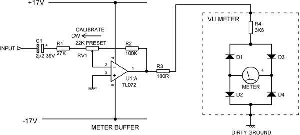
Figure 18.3: A very simple but effective design for a VU meter buffer stage
Because of their slow response, VU meters are sometimes made with a Peak LED projecting through the meter scale. This is driven by a peak-detect circuit of the sort described earlier in this chapter.
PPM Meters
Peak program meters (PPMs) are essentially peak-reading instruments that respond much more quickly than VU meters. They are always a good deal more expensive, partly because of the precisely defined and rather demanding characteristics of the physical meter itself – for example, the needle has to be able to move much faster than a VU needle, but without excessive overshoot – and partly because they need much more complex drive circuitry. The PPM standard was originally developed by the BBC in 1938, as a response to the inadequacy of existing average-responding meters. PPMs have a distinctive scale with white legends and a white needle against a black background, and are marked from 1 to 7. This is a logarithmic scale giving 4 decibels per division, and the accurate and temperature-stable implementation of this characteristic is what makes the drive circuitry expensive.
Nonetheless PPMs are specifically designed not to catch the very fastest of transient peaks, and are therefore sometimes called ‘quasi-peak’ meters. They only respond to transients sustained for a defined time; the specs give ‘type I’ meters an integration time of 5 ms, while ‘type II’ meters use 10 ms. The result is that transient levels normally exceed the PPM reading by some 4–6 dB. This approach encourages operators to somewhat increase program levels, giving a better signal-to-noise performance. The assumption (which is generally well-founded) is that occasional clipping of brief transients is not audible. The existence of both type I and II meters simply reflects differing views on the audibility of transient distortion.
PPMs exhibit a slow fallback from peak deflections, so it is easier to read peak levels visually. Type I meters should take 1.4–2.0 seconds to fall back 20 dB, while type II meters should take 2.5–3.1 seconds to fall back 24 dB. Type II meters also incorporate a delay of 75–150 ms before the needle fallback is allowed to begin; this peak-hold action makes reading easier.
LED Bar-Graph Metering
Bar-graph meters are commonly made up of an array of LEDs. An LED bar-graph meter can be made effectively with an active-rectifier circuit and a resistive divider chain that sets up the trip voltage of an array of comparators; this allows complete freedom in setting the trip level for each LED. A typical circuit that indicates from 0 to −14 dB in 2-dB steps with a selectable peak or average-reading characteristic is shown in Figure 18.4 and illustrates some important points in bar-graph design.
U3 is a half-wave precision rectifier of a familiar type, where negative feedback servos out the forward drop of D11, and D10 prevents op-amp clipping when D11 is reverse-biased. The rectified signal appears at the cathode of D11, and is smoothed by R7 and C1 to give an average, sort-of-VU response. D12 gives a separate rectified output and drives the peak-storage network R10, C9, which has a fast attack and a slow decay through R21. Either average or peak outputs are selected by SW1, and applied to the non-inverting inputs of an array of comparators. The LM2901 quad voltage comparator is very handy in this application; it has low input offsets and the essential open-collector outputs.
The inverting comparator inputs are connected to a resistor divider chain that sets the trip level for each LED. With no signal input, the comparator outputs are all low and their open-collector outputs shunt the LED chain current from Q1 to −15 V, so all LEDs are off. As the input signal rises in level, the first comparator U2:D switches its output off, and LED D8 illuminates. With more signal, U2:C also switches off and D7 comes on, and so on, until U1:A switches off and D1 illuminates. The important points about the LED chain are that the highest level LED is at the bottom of the chain, as it comes on last, and that the LED current flows from one supply rail down to the other, and is not passed into a ground. This prevents noise from getting into the audio path. The LED chain is driven with a constant-current source to keep LED brightness constant despite varying numbers of them being in circuit; this uses much less current than giving each LED its own resistor to the supply rail, and is universally used in mixing console metering. Make sure you have enough voltage headroom in the LED chain, not forgetting that yellow and green LEDs have a larger forward drop than red ones. The circuit shown has plenty of spare voltage for its LED chain, and so it is possible to put other indicator LEDs in the same constant-current path; for example, D9 can be switched on and off completely independently of the bar-graph LEDs, and can be used to indicate Channel On status or whatever. An important point is that in use the voltage at the top of the LED chain is continually changing in 2-V steps, and this part of the circuit must be kept away from the audio path to prevent horrible crunching noises from crosstalking into it.
This meter can of course be modified to have a different number of steps, and there is no need for the steps to be the same size. It is as accurate in its indications as the use of E24 values in the resistor divider chain allows.
If a lot of LED steps are required, there are some handy ICs that contain multiple open-collector comparators connected to an in-built divider chain. The National LM3914 has 10 comparators and a divider chain with equal steps, so they can be daisy-chained to make big displays, but some law bending is required if you want a logarithmic output. The National LM3915 also has 10 comparators, but a logarithmic divider chain covering a 30 dB range in 3-dB steps.
A More Efficient LED Bar-Graph Architecture
The bar-graph meter shown in Figure 18.4 above draws 6 mA from the two supply rails at all times, even if all the LEDs are off for long periods, which is often the case in recording work. This is actually desirable in a simple mixer as the ±15 or ±17 V rails are also used to power the audio circuitry, and step-changes in current taken by the meter could get into the ground system via decoupling capacitors and suchlike, causing highly unwelcome clicks.
In larger mixers a separate meter supply is provided to prevent this problem, and this allows more freedom in the design of the meter circuitry. In the example I am about to recount, the meter supply available was a single rail of +24 V; this came from an existing power supply design and was not open to alteration, negotiation or messing about with. A meter design with 20 LEDs was required, and an immediate problem was that you cannot power 20 LEDs of assorted colors with one chain running from +24 V; two LED chains would be required and the power consumption of the meter, even when completely dormant, would be twice as great. I therefore devised a more efficient system, which not only saves a considerable amount of power, but also actually economizes on components.
The meter circuit is shown in Figure 18.5, and I must admit it is not one of those circuit diagrams where the modus operandi exactly leaps from the page. However, stick with me.

Figure 18.5: A more efficient LED bar-graph meter
There are two LED chains, each powered by its own constant-current source Q1, Q2. The relevant current source is only turned on when it is needed. With no signal input, all LEDs are off; the outputs of comparators U10 and U20 are high (open-collector output off) and both Q1 and Q2 are off. The outputs of all other comparators are low. When a steadily increasing signal arrives, U20 is the first comparator to switch, and LED D20 turns on. With increasing signal, the output of U19 goes high, and the next LED, D19, turns on. This continues in exactly the same way as the conventional bar-graph circuit described above until all the LEDs in the chain D11–D20 are illuminated. As the signal increases further, comparator U10 switches and turns on the second current source Q2, illuminating D10; the rest of the LEDs in the second chain are then turned on in sequence as before. This arrangement saves a considerable amount of power, as no supply current at all is drawn when the meter is inactive, and only half the maximum is drawn so long as the indication is below −2 dB.
There are 10 comparators for each LED chain, 20 in all, so a long potential divider with 21 resistors would be required to provide the reference voltage for each comparator if it was done in the conventional way, as shown in Figure 18.4. However, looking at all those comparator inputs tied together, it struck me there might be a better way to generate all the reference voltages required, and there is.
The new method, which I call a ‘matrix divider’ system, uses only 10 resistors. This is more significant than it might at first appear, because the LEDs are on the edge of the PCB, the comparators are in compact quad packages, and so the divider resistors actually take up quite a large proportion of the PCB area. Reducing their number by half made fitting the meter into a pre-existing and rather cramped meter bridge design possible without recourse to surface-mount techniques. There are now two potential dividers. Divider A is driven by the output of the rectifier circuit, while divider B produces a series of fixed voltages with respect to the +8.0 V sub-rail. As the input signal increases, the output of the meter rectifier goes straight to comparators U16–U20, which take their reference voltages from divider B and turn on in sequence as described above. Comparators U11–U15 are fed with the same reference voltages from divider B, but their signal from the meter rectifier is attenuated by divider A, coming from the tap between R3 and R5, and so these comparators require more input signal to turn on. This process is repeated for the third bank of comparators U6–U10, whose input signal is further attenuated, and finally for the fourth bank of comparators U1–U5, whose input is still further attenuated. The result is that all the comparators switch in the correct order.
Since in this application there was a only single supply rail, a bias generator is required to generate an intermediate sub-rail to bias the op-amps. This sub-rail is set at +8.0 V rather than V/2, to allow enough headroom for the rectifier circuit, which produces only positive outputs; it is generated by R18, R19 and C3, and buffered by op-amp section U3:B. The main +24 V supply is protected by a 10 Ω fusible resistor R22, so if a short-circuit occurs on the meter PCB the resistor will fail open and the whole metering system will not be shut down. This kind of per-module fusing is very common and very important in mixer design; it localizes a possibly disabling fault to one module, and avoids having the power supply shut down, which would put the whole mixer out of action. A small but vital point is that the supply for divider B is taken from outside this fusing resistor; if it was not the divider voltages would vary with the number of LED chains powered, upsetting meter accuracy.
Once again the LM2901 quad voltage comparator is used, as it has low input offset voltages and the requisite open-collector outputs. Q1, Q2 can be any TO-92 devices with reasonable beta; their maximum power dissipation, which occurs with only one LED on in the chain, is a modest 128 mW. This meter system was used with great success.
Vacuum Fluorescent Displays
Vacuum fluorescent displays are sometimes used but require hefty tooling charges if you want a custom display, and their high-voltage operation makes driving them more complicated. The main power supply is usually 250 V DC, a voltage that requires considerable respect.
LCD Meter Displays
The ultimately versatile metering system is provided by making the meter display from a number of color LCD display screens. These can be of the size used in the smaller laptop computers, butted side-to-side to make something like a conventional meterbridge, or larger screens that can show three or more rows of bar-graphs at once. All the Calrec digital consoles currently have such metering. The advantages are obviously that you can display any kind of metering that you can think up, and the technology can be based on standard graphics cards.
Small Signal Audio Design; ISBN: 9780240521770
Copyright © 2010 Elsevier Ltd; All rights of reproduction, in any form, reserved.