
LEARNING OBJECTIVES
To appreciate the use of quantitative, objective approaches to software cost estimation
To have insight into the factors that affect software development productivity
To understand well-known techniques for estimating software cost and effort
To understand techniques for relating effort to development time
Note
Software development takes time and money. When commissioning a building project, you expect a reliable estimate of the cost and development time up front. Getting reliable cost and schedule estimates for software development projects is still largely a dream. Software development costs are notoriously difficult to estimate reliably at an early stage. Since progress is difficult to 'see' – just when is a piece of software 50% complete? – schedule slippages often go undetected for quite a while and schedule overruns are the rule, rather than the exception. In this chapter, we look at various ways to estimate software cost and schedule.
When commissioning someone to build a house, decorate a bathroom, or lay out a garden, we expect a precise estimate of the costs to be incurred before the operation is started. A gardener is capable of giving a rough indication of the cost on the basis of, say, the area of land, the desired size of the terrace or grass area, whether or not a pond is required, and similar information. The estimate can be made more precise in further dialog, before the first bit of earth is turned. If you expect similar accuracy as regards the cost estimate for a software development project, you are in for a surprise.
Estimating the cost of a software development project is a field in which one all too often relies on mere guesswork. There are exceptions to this procedure, though. There exist a number of algorithmic models that allow us to estimate total cost and development time of a software development project, based on estimates for a limited number of relevant cost drivers. Some of the important algorithmic cost estimation models are discussed in Section 7.1.
In most cost estimation models, a simple relation between cost and effort is assumed. The effort may be measured in man-months, for instance, and each man-month is taken to incur a fixed amount, say, of $5000. The total estimated cost is then obtained by simply multiplying the estimated number of man-months by this constant factor. In this chapter, we freely use the terms cost and effort as if they are synonymous.
The notion of total cost is usually taken to indicate the cost of the initial software development effort, i.e. the cost of the requirements engineering, design, implementation and testing phases. Thus, maintenance costs are not taken into account. Unless explicitly stated otherwise, this notion of cost will also be used by us. In the same vein, development time will be taken to mean the time between the start of the requirements engineering phase and the point in time when the software is delivered to the customer. The notion of cost as it is used here does not include possible hardware costs either. It concerns only personnel costs involved in software development.
Research in the area of cost estimation is far from crystallized. Different models use different measures and cost drivers, so that comparisons are very difficult. Suppose some model uses an equation of the form:
This equation shows a certain relation between effort needed (E) and the size of the product (KLOC = Kilo Lines Of Code = Lines Of Code /1 000). The effort measure could be the number of man-months needed. Several questions come to mind immediately: What is a line of code? Do we count machine code or the source code in some high-level language? Do we count comment lines and blank lines that increase readability? Do we take into account holidays, sick-leave, and so on, in our notion of the man-month or does it concern a net measure? Different interpretations of these notions may lead to widely different results. Unfortunately, different models do use different definitions of these notions. Sometimes, it is not even known which definitions were used in the derivation of the model.
To determine the equations of an algorithmic cost estimation model, we may follow several approaches. We may base our equations on the results of experiments. In such an experiment, we vary one parameter, while keeping the other parameters constant. In this way, we may try to determine the influence of the parameter that is being varied. As a typical example, we may consider the question of whether or not comments help to build up our understanding of a program. Under careful control of the circumstances, we may pose a number of questions about the same program text to two groups of programmers. The first group gets program text without comments, the second group gets the same program text with comments. We may check our hypothesis using the results of the two groups. The, probably realistic, assumption in this experiment is that a better and faster understanding of the program text has a positive effect on the maintainability of that program. This type of laboratory experiment is often performed at universities, where students play the role of programmers. It is not self-evident that the results thus obtained also hold in industrial settings. In practice, there may be a rather complicated interaction between relevant factors. Also, the subjects may not be representative. Finally, the generalization from laboratory experiments that are (of necessity) limited in size to the big software development projects with which professionals are confronted is not possible. The general opinion is that results thus obtained have limited validity and certainly need further testing.
A second way to arrive at an algorithmic cost estimation model is based on an analysis of real project data, in combination with some theoretical underpinning. An organization may collect data about a number of software systems that have been developed. This data may concern the time spent on the various phases that are distinguished, the qualifications of the personnel involved, the points in time at which errors occurred, both during testing and after installation, the complexity, reliability and other relevant project factors, the size of the resulting code, etc. Based on a sound hypothesis of the relations between the various entities involved and a (statistical) analysis of this data, we may derive equations that numerically characterize these relations. An example of such a relation is the one given above, which relates E to KLOC. The usability and reliability of such equations is obviously very much dependent upon the reliability of the data on which they are based. Also, the hypothesis that underlies the form of the equation must be sound.
Findings obtained in this way reflect an average, a best possible approximation based on available data. We therefore have to be very careful in applying the results obtained. If the software to be developed in the course of a new project cannot be compared with earlier products because of the degree of innovation involved, we are in for a big surprise. For example, estimating the cost of the Space Shuttle project cannot be done through a simple extrapolation from earlier projects. We may hope, however, that the average software development project has a higher predictability as regards effort needed and the corresponding cost.
The way in which we obtain quantitative relations implies further constraints on the use of these models. The model used is based on an analysis of data from earlier projects. Application of the model to new projects is possible only insofar as those new projects resemble the projects on whose data the model is based. If we have collected data on projects of a certain kind and within a particular organization, a model based on this data cannot be used without amendment for different projects in a different organization. A model based on data about administrative projects in a government environment has little predictive value for the development of real-time software in the aerospace industry. This is one of the reasons why the models of, for example, Walston and Felix (1977) and Boehm (1981) (see Section 7.1 for more detailed discussions of these models) yield such different results for the same problem description.
The lesson to be learned is that blind application of the formulae from existing models will not solve your cost estimation problem. Each model needs tuning to the environment in which it is going to be used. This implies the need to continuously collect your own project data and to apply statistical techniques to calibrate model parameters.
Other reasons for the discrepancies between existing models are:
Most models give a relation between man-months needed and size (in lines of code). As remarked before, widely different definitions of these notions are used.
The notion 'effort' does not always mean the same thing. Sometimes, one only counts the activities starting from the design, i.e. after the requirements specification has been fixed. Sometimes one also includes maintenance effort.
Despite these discrepancies, the various cost estimation models do have a number of characteristics in common. These common characteristics reflect important factors that bear on development cost and effort. The increased understanding of software costs allows us to identify strategies for improving software productivity, the most important of which are:
Writing less code. System size is one of the main determinants of effort and cost. Techniques that try to reduce size, such as software reuse and the use of high-level languages, can obtain significant savings.
Getting the best from people. Individual and team capabilities have a large impact on productivity. The best people are usually a bargain. Better incentives, better work environments, training programs, and so on provide further productivity improvement opportunities.
Avoiding rework. Studies have shown that considerable effort is spent redoing earlier work. The application of prototyping or evolutionary development process models and the use of modern programming practices (such as information hiding) can yield considerable savings.
Developing and using integrated project support environments. Tools can help us eliminate steps or make steps more efficient.
In Section 7.1, we discuss and compare some of the well-known algorithmic models for cost estimation. In many organizations, software cost is estimated by human experts, who use their expertise and gut feeling, rather than a formula, to arrive at a cost estimate. Some of the dos and don'ts of expert-based cost estimation are discussed in Section 7.2.
Given an estimate of the size of a project, we are interested in the development time needed. We may conjecture that a project with an estimated effort of 100 man-months can be completed in one year with a team of 8.5 people or equally well in one month with a team of 100 people. This view is too naive. A project of a certain size corresponds to a certain nominal physical time period. If we try to shorten this nominal development time too much, we get into the 'impossible region' and the chance of failure sharply increases. This phenomenon is further discussed in Section 7.3.
The models discussed in Section 7.1 fit planning-driven development projects more than they do agile projects. And even for planning-driven projects, their value is disputed, since the size of the project is unknown when the estimate is needed. It is like the story about a man who has lost his keys in a dark place going to search for them under a lamp, since this is the only place with enough light for searching. These models do have value, though, for the insights they offer into which factors influence productivity. If we compare successive versions of models, such as COCOMO and COCOMO 2, we also get insight into how these productivity factors have changed over time.
In agile projects (see Chapter 3), iterations are usually fairly small and the increments correspond to one or a few user stories or scenarios. These user stories are estimated in terms of development weeks, dollars, or some artificial unit, such as 'Points'. Then it is determined which user stories will be realized in the current increment and development proceeds. Often, the agreed time box is sacrosanct: if some of the user stories cannot be realized within the agreed upon time frame, they are moved to a later iteration. Estimation accuracy is assumed to improve in the course of the project. Cost estimation for agile projects is discussed in Section 7.4.
To be able to get reliable estimates, we need to record historical data extensively. This historical data can be used to produce estimates for new projects. In doing so, we predict the expected cost due to measurable properties of the project at hand. Just as the cost of laying out a garden might be a weighted combination of a number of relevant attributes (size of the garden, size of the grass area, whether there is a pond), so we would like to estimate the cost of a software development project. In this section, we discuss efforts to get algorithmic models to estimate software cost.
In the introduction to this chapter, we noticed that programming effort is strongly correlated with program size. There exist various (non-linear) models which express this correlation. A general form is
Here, KLOC again denotes the size of the software (lines of code/1 000), while E denotes the effort in man-months. a, b and c are constants, and f(x1, ..., xn) is a correction which depends on the values of the entities x1, ..., xn. In general, the base formula
is obtained through regression analysis of available project data. Thus, the primary cost driver is software size, measured in lines of code. This nominal cost estimate is tuned by correcting it for a number of factors that influence productivity (so-called cost drivers). For instance, if one of the factors used is 'experience of the programming team', this could incur a correction to the nominal cost estimate of 1.50, 1.20, 1.00, 0.80 and 0.60 for very low, low, average, high and very high levels of expertise, respectively.
Table 7.1 contains some of the well-known base formulae for the relation between software size and effort. For reasons mentioned before, it is difficult to compare these models. It is interesting to note, though, that the value of c fluctuates around 1 in most models.
Table 7.1. Formulae for the relation between size and effort
Origin | Base formula | See section |
|---|---|---|
Halstead | E = 0.7KLOC1.50 | 12.1.4 |
Boehm | E = 2.4KLOC1.05 | 7.1.2 |
Walston–Felix | E = 5.2KLOC0.91 | 7.1.1 |
This phenomenon is well known from the theory of economics. In a so-called economy of scale, one assumes that it is cheaper to produce large quantities of the same product. The fixed costs are then distributed over a larger number of units, which decreases the cost per unit. We thus realize an increasing return on investment. In the opposite case, we find a diseconomy of scale: after a certain point the production of additional units incurs extra costs.
In the case of software, the lines of code are the product. If we assume that producing a lot of code will cost less per line of code, formulae such as that of Walston—Felix (where c < 1) result. This may occur, for example, because the cost of expensive tools such as program generators, programming environments and test tools can be distributed over a larger number of lines of code. Alternatively, we may reason that large software projects are more expensive, relatively speaking. There is a larger overhead because of the increased need for communication and management control, because of the problems and interfaces getting more complex, and so on. Thus, each additional line of code requires more effort. In such cases, we obtain formulae such as those of Boehm and Halstead (where c > 1). There is no really convincing argument for either type of relation, though the latter (c > 1) may seem more plausible. Certainly for large projects, the effort required does seem to increase more than linearly with size.
It is clear that the value of the exponent c strongly influences the computed value E, certainly for large values of KLOC. Table 7.2 gives the values for E, as they are computed for the models of Table 7.1 and some values for KLOC. The reader will notice large differences between the models. For small programs, Halstead's model yields the lowest cost estimates. For projects in the order of one million lines of code, this same model yields a cost estimate which is an order of magnitude higher than that of Walston—Felix.
Table 7.2. E versus KLOC for various base models
KLOC | E = 0.7KLOC1.50 | E = 2.4KLOC1.05 | E = 5.2KLOC0.91 |
|---|---|---|---|
1 | 0.7 | 2.4 | 5.2 |
10 | 22.1 | 26.9 | 42.3 |
50 | 247.5 | 145.9 | 182.8 |
100 | 700.0 | 302.1 | 343.6 |
1 000 | 22 135.9 | 3 390.1 | 2 792.6 |
However, we should not immediately conclude that these models are useless. It is much more likely that there are big differences in the characteristics between the sets of projects on which the various models are based. Recall that the actual numbers used in those models result from an analysis of real project data. If this data reflects widely different project types or development environments, so will the models. We cannot simply copy those formulae. Each environment has its own specific characteristics and tuning the model parameters to the specific environment (a process called calibration) is necessary.
The most important problem with this type of model is to get a reliable estimate of the software size early on. How should we estimate the number of pages in a novel not yet written? Even if we know the number of characters, the number of locations and the time interval in which the story takes place, we should not expect a realistic size estimate up front. The further advanced we are with the project, the more accurate our size estimate will get. If the design is more or less finished, we may (possibly) form a reasonable impression of the size of the resulting software. Only if the system has been delivered, do we know the exact number.
The customer, however, needs a reliable cost estimate early on. In such a case, lines of code is a measure which is too inexact to act as a basis for a cost estimate. We therefore have to look for an alternative. In Section 7.1.4 we discuss a model based on quantities, which are known at an earlier stage.
We may also switch to another model during the execution of a project, since we may expect to get more reliable data as the project is making progress. We then get a cascade of increasingly detailed cost estimation models. COCOMO 2 is an example of this (see Section 7.1.5).
The base equation of the model derived by Walston and Felix (1977) is
Some 60 projects from IBM were used in the derivation of this model. These projects differed widely in size and the software was written in a variety of programming languages. It therefore comes as no surprise that the model, applied to a subset of these 60 projects, yields unsatisfactory results.
In an effort to explain these wide-ranging results, Walston and Felix identified 29 variables that clearly influenced productivity. For each of these variables, three levels were distinguished: high, average and low. For 51 projects, Walston and Felix determined the level of each of these 29 variables and the productivity obtained (in terms of lines of code per man-month). These results are given in Table 7.3 for some of the most important variables. Thus, the average productivity turned out to be 500 lines of code per man-month for projects with a user interface of low complexity. With a user interface of average or high complexity, the productivity is 295 and 124 lines of code per man-month, respectively. The last column contains the productivity change PC, the absolute value of the difference between the high and low scores.
According to Walston and Felix, a productivity index I can now be determined for a new project, as follows:
The weights Wi are defined by
Here, PCi is the productivity change of factor i. For the first factor from Table 7.3 (complexity of the user interface), the following holds: PC1 = 376, so W1 = 1.29. The variables Xi can take on values +1, 0 and −1, where the corresponding factor scores as low, average or high (and thus results in a high, average or low productivity, respectively). The productivity index obtained can be translated into an expected productivity (lines of code produced per man-month). Details of the latter are not given in (Walston and Felix, 1977).
The number of factors considered in this model is rather high (29 factors from 51 projects). It is not clear to what extent the various factors influence each other. Finally, the number of alternatives per factor is only three, which does not seem to offer enough choice in practical situations.
Nevertheless, the approach taken by Walston and Felix and their list of cost drivers have played a very important role in directing later research in this area.
Table 7.3. Productivity intervals (Source: C.E. Walston and C.P. Felix, A method for programming measurement and estimation, IBM Systems Journal, © 1977.)
Variable | Value of variable average productivity (LOC) | | high – low | (PC) | ||
|---|---|---|---|---|
Complexity of user interface | <normal 500 | normal 295 | >normal 124 | 376 |
User participation during requirements specification | none 491 | some 267 | much 205 | 286 |
User-originated changes in design | few 297 | – | many 196 | 101 |
User-experience with | none 318 | some 340 | much 206 | 112 |
Qualification, experience of personnel | low 132 | average 257 | high 410 | 278 |
Percentage programmers participating in design | <25% 153 | 25–50% 242 | >50% 391 | 238 |
Previous experience with operational computer | minimal 146 | average 270 | extensive 312 | 166 |
Previous experience with programming languages | minimal 122 | average 225 | extensive 385 | 263 |
Previous experience with application of similar or greater size and complexity | minimal 146 | average 221 | extensive 410 | 264 |
Ratio of average team size to duration (people/month) | <0.5 305 | 0.5–0.9 310 | >0.9 171 | 134 |
The COnstructive COst MOdel (COCOMO) is one of the best-documented algorithmic cost estimation models. In its simplest form, Basic COCOMO, the formula that relates effort to software size, reads
Here, b and c are constants that depend on the kind of project that is being executed. COCOMO distinguishes three classes of project:
Organic A relatively small team develops software in a known environment. The people involved generally have a lot of experience with similar projects in their organization. They are thus able to contribute at an early stage, since there is no initial overhead. Projects of this type will seldom be very large projects.
Embedded The product will be embedded in an environment which is very inflexible and poses severe constraints. An example of this type of project might be air traffic control or an embedded weapons system.
Semidetached This is an intermediate form. The team may include a mixture of experienced and inexperienced people, the project may be fairly large, though not excessively large, etc.
For the various classes of project, the parameters of Basic COCOMO take on the following values:
Equation 7.7.
Table 7.4 gives the estimated effort for projects of each of those three modes, for different values of KLOC (though an 'organic' project of one million lines is not very realistic). Amongst other things, we may read from this table that the constant c soon starts to have a major impact on the estimate obtained.
Table 7.4. Size versus effort in Basic COCOMO
KLOC | Organic (E = 2.4KLOC1.05) | Effort in man-months Semidetached (E = 3.0KLOC1.12) | Embedded (E = (E = 3.6KLOC1.20) |
|---|---|---|---|
1 | 2.4 | 3.0 | 3.6 |
10 | 26.9 | 39.6 | 57.1 |
50 | 145.9 | 239.4 | 392.9 |
100 | 302.1 | 521.3 | 904.2 |
1 000 | 3 390.0 | 6 872.0 | 14 333.0 |
Basic COCOMO yields a simple, and hence a crude, cost estimate based on a simple classification of projects into three types. Boehm (1981) also discusses two other, more complicated, models called Intermediate COCOMO and Detailed COCOMO. Both these models take into account 15 cost drivers – attributes that affect productivity, and hence costs.
All these cost drivers yield a multiplicative correction factor to the nominal estimate of the effort. (Both these models also use values for b which slightly differ from that of Basic COCOMO.) Suppose we find a nominal effort estimate of 40 man-months for a certain project. If the complexity of the resulting software is low, then the model tells us to correct this estimate by a factor of 0.85. A better estimate then would be 34 man-months. On the other hand, if the complexity is high, we get an estimate of 1.15 × 40 = 46 man-months.
The nominal value of each cost driver in Intermediate COCOMO is 1.00 (see also Table 7.10). So we may say that Basic COCOMO is based on nominal values for each of the cost drivers.
The COCOMO formulae are based on a combination of expert judgment, an analysis of available project data, other models, and so on. The basic model does not yield very accurate results for the projects on which the model has been based. The intermediate version yields good results and, if one extra cost driver (volatility of the requirements specification) is added, it even yields very good results. Further validation of the COCOMO models using other project data is not straightforward, since the necessary information to determine the ratings of the various cost drivers is, in general, not available. So we are left only with the ability to test the basic model. Here, we obtain fairly large discrepancies between the effort estimated and the actual effort needed.
An advantage of COCOMO is that we know all its details. A major update of the COCOMO model, better reflecting current and future software practices, is discussed in Section 7.1.5.
Norden studied the distribution of manpower over time in a number of software development projects in the 1960s. He found that this distribution often had a very characteristic shape which is well-approximated by a Rayleigh distribution. Based upon this finding, Putnam (1978) developed a cost estimation model in which the manpower required (MR) at time t is given by
where a is a speed-up factor which determines the initial slope of the curve, while K denotes the total manpower required, including in the maintenance phase. K equals the volume of the area delineated by the Rayleigh curve (see Figure 7.1).
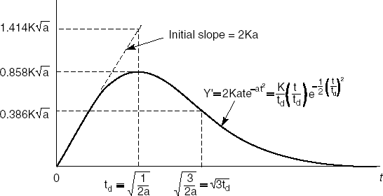
Figure 7.1. The Rayleigh curve for software schedules (Source: M.L. Shooman, Tutorial on software cost models, IEEE Catalog nr TH0067-9, © 1979 IEEE. Reproduced with permission.)
The shape of this curve can be explained theoretically as follows. Suppose a project consists of a number of problems for which a solution must be found. Let W(t) be the fraction of problems for which a solution has been found at time t. Let p(t) be the problem-solving capacity at time t. Progress at time t then is proportional to the product of the available problem-solving capacity and the fraction of problems yet unsolved. If the total amount of work to be done is set to 1, this yields:
After integration, we get
If we next assume that the problem-solving capacity is well approximated by an equation of the form p(t) = at, i.e. the problem-solving capacity shows a linear increase over time, the progress is given by a Rayleigh distribution:
Integration of the equation for MR(t) that was given earlier yields the cumulative effort I:
In particular, we get I(∞) = K. If we denote the point in time at which the Rayleigh curve assumes its maximum value by T, then a = 1/(2T2). This point T will be close to the point in time at which the software is being delivered to the customer. The volume of the area delineated by the Rayleigh curve between points 0 and T, then, is a good approximation of the initial development effort. For this, we get
This result is remarkably close to the often-used rule of thumb: 40% of the total effort is spent on the actual development, while 60% is spent on maintenance.
Various studies indicate that Putnam's model is well suited to estimating the cost of very large software development projects (projects that involve more than 15 man-years). The model seems to be less suitable for small projects.
A serious objection to Putnam's model, in our opinion, concerns the relation it assumes between effort and development time if the schedule is compressed relative to the nominal schedule estimate: E = c/T4. Compressing a project's schedule in this model entails an extraordinarily large penalty (see also Section 7.3).
Function point analysis (FPA) is a method of estimating costs in which the problems associated with determining the expected amount of code are circumvented. FPA is based on counting the number of data structures that are used. In the FPA method, it is assumed that the number of data structures is a good size indicator. FPA is particularly suitable for projects aimed at realizing business applications, in which the structure of the data plays a very dominant role. The method is less suited to projects in which the structure of the data plays a less prominent role and the emphasis is on algorithms (such as compilers and most real-time software).
The following five entities play a central role in the FPA model:
Number of input types (I). The input types refer only to user input that results in changes in data structures. It does not refer to user input which is solely concerned with controlling the program's execution. Each input type that has a different format, or is treated differently, is counted. Although the records of a master file and those of a mutation file may have the same format, they are still counted separately.
Number of output types (O). For the output types, the same counting scheme as for the input types is used.
Number of inquiry types (E). Inquiry types concern input that controls the execution of the program and does not change internal data structures. Examples of inquiry types are menu selections and query criteria.
Number of logical internal files (L). This concerns internal data generated by the system, and used and maintained by the system, such as, for example, an index file.
Number of interfaces (F). This concerns data that is output to another application or is shared with some other application.
By trial and error, weights have been associated with each of these entities. The number of (unadjusted) function points, UFP, is a weighted sum of these five entities:
With FPA too, a further refinement is possible, by applying corrections to reflect differences in complexity of the data types. In that case, the constants used in the above formula depend on the estimated complexity of the data type in question. Table 7.5 gives the counting rules when three levels of complexity are distinguished. So, rather than having each input type count as four function points, we may count three, four or six function points, based on an assessment of the complexity of each input type.
Table 7.5. Counting rules for (unadjusted) function points
Type | Complexity level | ||
|---|---|---|---|
Simple | Average | Complex | |
Input (I) | 3 | 4 | 6 |
Output (O) | 4 | 5 | 7 |
Inquiry (E) | 3 | 4 | 6 |
Logical internal (L) | 7 | 10 | 15 |
Interfaces (F) | 5 | 7 | 10 |
Each input type has a number of data element types (attributes) and refers to zero or more other file types. The complexity of an input type increases as the number of its data element types or referenced file types increases. For input types, the mapping of these numbers to complexity levels is given in Table 7.6. For the other file types, these tables have the same format, with slightly different numbers along the axes.
Table 7.6. Complexity levels for input types
# of file types | # of data elements | ||
|---|---|---|---|
1–4 | 5–15 | >15 | |
0 or 1 | simple | simple | average |
2–3 | simple | average | complex |
>3 | average | complex | complex |
As in other cost estimation models, the unadjusted function point measure is adjusted by taking into account a number of application characteristics that influence development effort. Table 7.7 contains the 14 characteristics used in the FPA model. The degree of influence of each of these characteristics is valued on a six-point scale, ranging from zero (no influence, not present) to five (strong influence). The total degree of influence DI is the sum of the scores for all characteristics. This number is then converted to a technical complexity factor (TCF) using the formula
Table 7.7. Application characteristics in FPA
|
The (adjusted) function point measure, FP, is now obtained through
Finally, there is a direct mapping from the (adjusted) function points to lines of code. For instance, in (Albrecht, 1979) one function point corresponds to 65 lines of PL/I or 100 lines of COBOL, on average.
In FPA, it is not simple to decide exactly when two data types should be counted as separate. Also, the difference between, for example, input types, inquiry types, and interfaces remains somewhat vague. The International Function Point User Group (IFPUG) has published extensive guidelines on how to classify and count the various entities involved. This should overcome many of the difficulties that analysts have in counting function points in a uniform way.
Further problems with FPA have to do with its use of ordinal scales and the way complexity is handled. FPA distinguishes only three levels of component complexity. A component with 100 elements thus gets at most twice the number of function points as a component with one element. It has been suggested that a model which uses the raw complexity data, i.e. the number of data elements and file types referenced, might work as well as, or even better than, a model which uses an ordinal derivative thereof. In a sense, complexity is counted twice: both through the complexity level of the component and through one of the application characteristics. Yet it is felt that highly complex systems are not adequately dealt with, since FPA is predominantly concerned with counting externally visible inputs and outputs.
In applying the FPA cost estimation model, it still remains necessary to calibrate the various entities to your own environment. This holds even more for the corrections that reflect different application characteristics and the transition from function points to lines of code.
COCOMO 2 is a revision of the 1981 COCOMO model, tuned to the life cycle practices of the 1990s and 2000s. It reflects our cumulative experience with and knowledge of cost estimation. By comparing its constituents with those of previous cost estimation models, it also offers us a way of learning about significant changes in our trade over the decades.
COCOMO 2 provides three increasingly detailed cost estimation models. These models can be used for different types of project, as well as during different stages of a single project:
The application composition model is mainly intended for prototyping efforts, for instance to resolve user interface issues. (Its name suggests heavy use of existing components, presumably in the context of a powerful CASE environment.)
The early design model is aimed at the architectural design stage.
The post-architecture model deals with the actual development stage of a software project.
The post-architecture model can be considered an update of the original COCOMO model; the early design model is an FPA-like model; and the application composition model is based on counting system components of large granularity, known as object points. Object points have nothing to do with objects as in object-oriented development. In this context, objects are screens, reports, and 3GL modules.
The roots of this type of model can be traced back to several variations on FPA-type size measures. Function points as used in FPA are intended to be a user-oriented measure of system function. The user functions measured are the inputs, outputs, inquiries, etc. We may conjecture that these user-functions are technology-dependent and that FPA primarily reflects the batch-oriented world of the 1970s.
Present-day administrative systems are perhaps better characterized by their numbers of menus or screens. This line of thought has been pursued in various studies. (Banker et al., 1991) compared object points with function points for a sample of software projects, and found that object points did almost as well as function points. Object points, however, are easier to determine and can be determined at an earlier point in time.
Total effort is estimated in the application composition model as follows:
Estimate the number of screens, reports, and 3GL components in the application.
Determine the complexity level of each screen and report (simple, medium or difficult). 3GL components are assumed to be always difficult. The complexity of a screen depends on the number of views and tables it contains. The complexity of a report depends on the number of sections and tables it contains. A classification table similar to those in FPA is used to determine the complexity level (see Table 7.8).
Use the numbers given in Table 7.9 to determine the relative effort (in object points) to implement the object.
The sum of the object points for the individual objects yields the number of object points for the whole system.
Estimate the reuse percentage, resulting in the number of new object points (NOP) as follows: NOP = ObjectPoints × (100 – %Reuse)/100.
Determine a productivity rate PROD = NOP/man-month. This productivity rate depends on the experience and capability of both the developers and the maturity of the CASE environment they use. It varies from 4 (very low) to 50 (very high).
Estimate the number of man-months needed for the project: E = NOP/PROD.
The early design model uses unadjusted function points (UFPs) as its basic size measure. These unadjusted function points are counted in the same way as they are counted in FPA. The unadjusted function points are then converted to source lines of code (SLOC), using a ratio SLOC/UFP which depends on the programming language used. In a typical environment, each UFP may correspond to, say, 91 lines of Pascal, 128 lines of C, 29 lines of C++, or 320 lines of assembly language. Obviously, these numbers are environment-specific.
The early design model does not use the FPA scheme to account for application characteristics. Instead, it uses a set of seven cost drivers, which are combinations of the full set of cost drivers of the post-architecture model (see Table 7.10). The intermediate, reduced set of cost drivers is:
product reliability and complexity, a combination of required software reliability, database size, product complexity and documentation needs
required reuse, which is equivalent to its post-architecture counterpart
platform difficulty, a combination of execution time, main storage constraints, and platform volatility
personnel experience, a combination of application, platform, and tool experience
personnel capability, a combination of analyst and programmer capability and personnel continuity
facilities, a combination of the use of software tools and multi-site development
schedule, which is equivalent to its post-architecture counterpart.
These cost drivers are rated on a seven-point scale, ranging from extra low to extra high. The values assigned are similar to those in Table 7.10. Thus, the nominal values are always 1.00 and the values become larger or smaller as the cost driver is estimated to deviate further from the nominal rating. After the unadjusted function points have been converted to thousands of source lines of code (KSLOC), the cumulative effect of the cost drivers is accounted for by the formula
The post-architecture is the most detailed model. Its basic effort equation is very similar to that of the original COCOMO model:
It differs from the original COCOMO model in its set of cost drivers, the use of lines of code as its base measure, and the range of values of the exponent b.
Table 7.10. Cost drivers and associated effort multipliers in COCOMO 2 (Source: B.W. Boehm et al., COCOMO II Model Definition Manual, University of Southern California, 1997. Reproduced with permission.)
Cost drivers | Rating | |||||
|---|---|---|---|---|---|---|
Very Low | Low | Nominal | High | Very high | Extra high | |
Product factors | ||||||
Reliability required | 0.75 | 0.88 | 1.00 | 1.15 | 1.39 | |
Database size | 0.93 | 1.00 | 1.09 | 1.19 | ||
Product complexity | 0.75 | 0.88 | 1.00 | 1.15 | 1.30 | 1.66 |
Required reusability | 0.91 | 1.00 | 1.14 | 1.29 | 1.49 | |
Documentation needs | 0.89 | 0.95 | 1.00 | 1.06 | 1.13 | |
Platform factors | ||||||
Execution-time constraints | 1.00 | 1.11 | 1.31 | 1.67 | ||
Main storage constraints | 1.00 | 1.06 | 1.21 | 1.57 | ||
Platform volatility | 0.87 | 1.00 | 1.15 | 1.30 | ||
Personnel factors | ||||||
Analyst capability | 1.50 | 1.22 | 1.00 | 0.83 | 0.67 | |
Programmer capability | 1.37 | 1.16 | 1.00 | 0.87 | 0.74 | |
Application experience | 1.22 | 1.10 | 1.00 | 0.89 | 0.81 | |
Platform experience | 1.24 | 1.10 | 1.00 | 0.92 | 0.84 | |
Language and tool experience | 1.25 | 1.12 | 1.00 | 0.88 | 0.81 | |
Personnel continuity | 1.24 | 1.10 | 1.00 | 0.92 | 0.84 | |
Project factors | ||||||
Use of software tools | 1.24 | 1.12 | 1.00 | 0.86 | 0.72 | |
Multi-site development | 1.25 | 1.10 | 1.00 | 0.92 | 0.84 | 0.78 |
Required development schedule | 1.29 | 1.10 | 1.00 | 1.00 | 1.00 | |
The differences between the COCOMO and COCOMO 2 cost drivers reflect major changes in the field. The COCOMO 2 cost drivers and the associated effort multipliers are given in Table 7.10. The values of the effort multipliers in this table are the result of calibration on a certain set of projects. The changes are as follows:
Four new cost drivers have been introduced: required reusability, documentation needs, personnel continuity, and multi-site development. They reflect the growing influence of those aspects on development cost.
Two cost drivers have been dropped: computer turnaround time and use of modern programming practices. Nowadays, developers use workstations, and (batch-processing) turnaround time is no longer an issue. Modern programming practices have evolved into the broader notion of mature software engineering practices, which are dealt with in the exponent b of the COCOMO 2 effort equation.
The productivity influence, i.e. the ratio between the highest and lowest value, of some cost drivers has been increased (analyst capability, platform experience, and language and tools experience) or decreased (programmer capability).
In COCOMO 2, the user may use both KSLOC and UFP as base measures. It is also possible to use UFP for part of the system. The UFP counts are converted to KSLOC counts as in the early design model, after which the effort equation applies.
Rather than having three 'modes', with slightly different values for the exponent b in the effort equation, COCOMO 2 has a much more elaborate scaling model. This model uses five scale factors Wi, each of which is rated on a six-point scale from very low (5) to extra high (0). The exponent b for the effort equation is then determined by the formula:
So, b can take values in the range 1.01 to 1.26, thus giving a more flexible rating scheme than that used in the original COCOMO model.
The scale factors used in COCOMO 2 are:
precedentedness, which indicates the novelty of the project to the development organization. Aspects such as experience with similar systems, the need for innovative architectures and algorithms, and the concurrent development of hardware and software are reflected in this factor.
development flexibility, which reflects the need for conformance with pre-established and external interface requirements and puts a possible premium on early completion.
architecture/risk resolution, which reflects the percentage of significant risks that have been eliminated. In many cases, this percentage will be correlated with the percentage of significant module interfaces specified, i.e. architectural choices made.
team cohesion, which accounts for possible difficulties in stakeholder interactions. This factor reflects aspects such as the consistency of stakeholder objectives and cultures, and the experience of the stakeholders in acting as a team.
process maturity, which reflects the maturity of the project organization according to the Capability Maturity Model (see Section 6.6).
Only the first two of these factors were, in a crude form, accounted for in the original COCOMO model.
The original COCOMO model allows us to handle reuse in the following way. The three main development phases, design, coding, and integration, are estimated to take 40%, 30%, and 30% of the average effort, respectively. Reuse can be catered for by separately considering the fractions of the system that require redesign (DM), recoding (CM), and re-integration (IM). An adjustment factor AAF is then given by the formula
An adjusted value AKLOC, given by
is used in the COCOMO formulae, instead of the unadjusted value KLOC. In this way, a lower cost estimate is obtained if part of the system is reused.
By treating reuse this way, it is assumed that developing reusable components does not require any extra effort. You may simply reap the benefits when part of a system can be reused from an earlier effort. This assumption does not seem to be very realistic. Reuse does not come for free (see also Chapter 17).
COCOMO 2 uses a more elaborate scheme to handle reuse effects. This scheme reflects two additional factors that impact the cost of reuse: the quality of the code being reused and the amount of effort needed to test the applicability of the component to be reused.
If the software to be reused is strongly modular and strongly matches the application in which it is to be reused, and the code is well-organized and properly documented, then the extra effort needed to reuse this code is relatively low, estimated to be 10%. This penalty may be as high as 50% if the software exhibits low coupling and cohesion, is poorly documented, and so on. This extra effort is denoted by the software understanding increment SU.
The degree of assessment and assimilation (AA) denotes the effort needed to determine whether a component is appropriate for the present application. It ranges from 0% (no extra effort required) to 8% (extensive test, evaluation and documentation required).
Both these percentages are added to the adjustment factor AAF, yielding the equivalent kilo number of new lines of code (EKLOC):
Function points, as discussed in Section 7.1.4, reflect transaction-oriented business applications from the 1970s. It may seem a bit odd to assume that the cost of modern, Web-based systems is determined by the number of input files, output files, and so on. On the other hand, it is an appealing idea to base the effort estimation on a small number of attributes of entities that are known at an early stage. The object points of COCOMO 2 are one example of this.
Another example is use-case points, which estimate effort based on a few characteristics of a set of use cases. The approach is very similar to that of FPA. First, the number of unadjusted use-case points (UUCP) is calculated. Next, this value is adjusted to cater for the complexity of the project (the technical complexity factor TCF) and the experience of the development team (the environmental complexity factor ECF). The formula thus reads
The value of UUCP depends on the complexity of the use case itself and the complexity of the actors involved. The use-case categories and actor classifications and their associated weights are given in Tables 7.11 and 7.12. Note the similarity with the way complexities are computed in FPA (Table 7.6). A few simple and easy-to-count attributes determine the weight used.
Table 7.11. Use case categories
Category | Weight | Description |
|---|---|---|
Simple | 5 | At most three steps in the success scenario; at most five classes in the implementation |
Average | 10 | Four to seven steps in the success scenario; five to ten classes in the implementation |
Complex | 15 | More than seven steps in the success scenario; more than ten classes in the implementation |
Table 7.12. Actor classifications
Category | Weight | Description |
|---|---|---|
Simple | 1 | Actor represents another system with a defined API |
Average | 2 | Actor represents another system interacting through a protocol |
Complex | 3 | Actor is a person interacting through an interface |
The technical complexity factor, TCF, is very similar to that of FPA. A number of factors is distinguished that may influence productivity of a project. Examples are whether or not the project is for a distributed system, whether or not special security features are needed, and so on. Overall, these technical factors more reflect characteristics of modern systems than those of Table 7.7. Altogether, TCF may reduce or enlarge the nominal effort expressed by UUCP by about 40%.
Table 7.13. Environmental complexity factors
Description | Weight |
|---|---|
Familiarity with UML | 1.5 |
Part-time workers | −1 |
Analyst capability | 0.5 |
Application experience | 0.5 |
Object-oriented experience | 1 |
Motivation | 1 |
Difficult programming language | −1 |
Stable requirements | 2 |
ECF works in a similar way. Table 7.13 lists the environmental complexity factors from (Clemmons, 2006). The factors 'Familiarity with UML' and 'Stable requirements' have a larger positive impact on effort than the others. Not surprisingly, 'Part-time workers' and 'Difficult programming language' have a negative impact. Again, a weight Wi and perceived value Fi is determined for each factor. The total impact is then given by
The range of Fi is 0 to 5. So the value of ECF ranges from 1.4 ('Part-time workers' and 'Difficult programming language' have weight 0, while the others have weight 5) to 0.425 (all weights are 0). ECF thus has a somewhat larger impact on effort than TCF.
Finally, UCP is translated into actual hours by multiplying it with some constant denoting the development hours per use-case point. This value depends on the local situation. It may be computed using statistics from previous projects. Typically, the number of hours per use-case point is in the range 15 to 30. Experience indicates that use-case point estimates deviate by at most 20% from actual effort.
Many of the models discussed in Section 7.1 are based on data about past projects. One of the main problems in applying these models is the sheer lack of quantitative data about past projects. There simply is not enough data available. Though the importance of such a database is now widely recognized, we still do not routinely collect data on current projects. It seems as if we cannot spare the time to collect data; we have to write software. DeMarco (1982) makes a comparison with the medieval barber who also acted as a physician. He could have made the same objection: 'We cannot afford the time to take our patient's temperature, since we have to cut his hair.'
We thus have to shift to other methods to estimate costs. These other methods are based on the expertise of the estimators. In doing so, certain traps have to be circumvented. It is particularly important to prevent political arguments from entering the arena. Typical political lines of reasoning are:
'We were given 12 months to do the job, so it will take 12 months.' This might be seen as a variation of Parkinson's Law: work fills the time available.
'We know that our competitor put in a bid of $1M, so we need to schedule a bid of $0.9M.' This is sometimes referred to as 'pricing to win.'
'We want to show our product at the trade show next year, so the software needs to be written and tested within the next nine months, though we realize that this is rather tight.' This could be termed the 'budget' method of cost estimation.
'Actually, the project needs one year, but I can't sell that to my boss. We know that ten months is acceptable, so we'll settle for ten months.'
Politically colored estimates can have disastrous effects, as has been shown all too often during the short history of our field. Political arguments almost always play a role if estimates are being given by people directly involved in the project, such as the project manager or someone reporting to the project manager. Very soon, then, estimates will influence, or be influenced by, the future assessment of those persons. To quote DeMarco (1982), 'one chief villain is the policy that estimates shall be used to create incentives'.
Jørgensen (2005) gives the following guidelines for expert-based effort estimation:
Do not mix estimation, planning, and bidding.
Combine estimation methods.
Ask for justification.
Select experts with experience from similar projects.
Accept and assess uncertainty.
Provide learning opportunities.
Consider postponing or avoiding effort estimation.
The politically colored lines of reasoning mentioned above all mix up estimation, planning, and bidding. However, they have different goals: estimation's only goal is accuracy; planning involves risk assessment and scheduling; and bidding is about winning a contract. Though these activities have different goals, they are of course related. A low bid, for instance, generally incurs a tight schedule and higher risks.
An interesting experiment on the effects of bidding on the remainder of a project is described in (Jørgensen and Grimstad, 2004). In this experiment, the authors study what is called the winner's curse, a phenomenon known from auctions, where players are uncertain of the value of an item when they bid. The highest bid wins, but the winner may be left with an item that's worth less than was paid for it. The term was first coined in the 1950s, when oil industries had no accurate way to estimate the value of their oil fields. In the software field, it has the following characteristics:
Software providers differ in optimism in their estimates of most likely cost: some are over-optimistic, some are realistic, and some are pessimistic.
Software providers with over-optimistic estimates tend to have the lowest bids.
Software clients require a fixed-price contract.
Software clients tend to select a provider with a low bid.
The result often is a Pyrrhic victory, a contract that results in low or negative profits to the bidder. But such a contract might also be risky for the client. Jørgensen and Grimstad (2004) describe an experiment in which they asked 35 companies for bids on a certain requirements specification. They then asked four companies to implement the system. They found that the companies with the lowest bids incurred the greatest risks.
Vacuuming a rug in two orthogonal directions is likely to pick up more dirt than vacuuming the rug twice in the same direction. Likewise, the combination of different estimation methods gives better estimates. So one may combine a COCOMO estimate with that of an expert, or estimates from experts with a different background. In this way, the bias that is inherent in a method or class of experts is mitigated.
Estimators should be held accountable for their estimates. Lederer and Prasad (2000) found that the use of estimates in performance evaluations of software managers and professionals is the only practice that leads to better estimates. In a slightly weaker form, one may at least ask for a justification of the estimate. Such a justification could refer to a calibrated model or a work breakdown structure in which cost estimates of components are derived from those in similar projects.
For lack of hard data, the cost of a software development project is often estimated through a comparison with earlier projects. If the estimator is very experienced, reasonable cost estimates may result. However, the learning effect of earlier experiences may lead to estimates that are too pessimistic in this case. Experience gained with a certain type of application may lead to higher productivity for subsequent projects. Similar applications thus give rise to lower costs.
McClure (1968) describes a situation in which a team was asked to develop a FORTRAN compiler for three different machines. The effort needed (in man-months) for these three projects is given in Table 7.14.
On the other hand, peculiar circumstances and particular characteristics of a specific project tend to get insufficient attention if cost is estimated through comparison with earlier projects. For example, a simple change of scale (automation of a local library with 25 000 volumes as opposed to a university library with over 1 000 000 volumes), slightly harsher performance requirements, a compressed schedule (which involves a larger team and thus incurs increased communication overheads) may have a significant impact on the effort required in terms of man-months. Careless application of the comparison method of cost estimation leads to estimates such as 'the cost of this project is equal to the cost of the previous project'.
Table 7.14. Learning effect of writing a FORTRAN compiler
Compiler | Number of man-months needed |
|---|---|
1 | 72 |
2 | 36 |
3 | 14 |
We may involve more than one expert in the estimation process. In doing so, each expert gives an estimate based on his own experience and expertise. Factors that are hard to quantify, such as personality characteristics and peculiar project characteristics, may thus be taken into account. Here too, the quality of the estimate cannot exceed the quality of the experts. The experts that participate in the estimate, then, should have experience in similar projects. It does not help all that much to ask an expert in office-automation systems to provide an estimate for an air-traffic-control system.
Estimates incur uncertainty. A cost estimate of, say, 100 man-months might mean that there is a 75% probability that the real cost of this project is between 80 and 120 man-months. It is not a point estimate. One method that aims to get a more reliable estimate is to have the expert produce more than one estimate. We all have the tendency to conceive an optimistic estimate as being realistic. (Have you ever heard of a software system being delivered ahead of time?) To obviate this tendency, we may employ a technique in which the expert is asked for three estimates: an optimistic estimate a, a realistic estimate m, and a pessimistic estimate b. Using a beta-distribution, the expected effort then is E = (a + 4m + b)/6. Though this estimate will probably be better than one based on the average of a and b, it seems justifiable to warn against too much optimism. Software has the tendency to grow and projects have the tendency to far exceed the estimated effort.
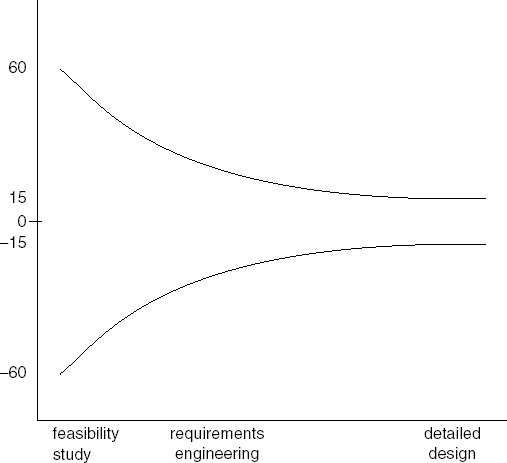
At the beginning of a project, the uncertainty is likely to be quite large. As a consequence, early cost estimates have a large range of uncertainty as well. As we progress to later phases, uncertainty decreases. For example, at the time of the feasibility study, the estimate may be 60% off, but the uncertainty may have decreased to 15% by the time the detailed design is ready (see Figure 7.2). After its shape, this is known as the 'cone of uncertainty'. In general, people considerably underestimate the size of the uncertainty interval (Jørgensen et al., 2004).
Training improves performance. This holds for skaters and it also applies to software cost estimators. Studies in other fields show that inexperienced people tend to overestimate their abilities and performance. There is no reason to expect the software field to be any different. The resulting cost and schedule overruns are all too common. Harrison (2004) suggests that a prime reason for more mature organizations to have fewer cost overruns is not so much higher productivity or better processes, but greater self-knowledge. I concur the same is true for people estimating software costs.
While executing a task, people have to make a number of decisions. These decisions are strongly influenced by requirements set or proposed. The cost estimate is one such requirement which will have an impact on the end result. We may imagine a hypothetical case in which model A estimates the cost at 300 man-months. Now suppose the project actually takes 400 man-months. If model B would have estimated the project at 450 man-months, is model B better than model A? It is quite possible that, starting from the estimate given by model B, the eventual cost would have been 600 man-months. The project's behavior is influenced by the cost estimate. Choices made during the execution of a project are influenced by cost estimates derived earlier. If a cost estimate is not needed, it is wise not to make one.
Having obtained an estimate of the total number of man-months needed for a given project, we are still left with the question of how many calendar months it will take. For a project estimated at 20 man-months, the kind of schedules you might think of, include:
20 people work on the project for 1 month;
4 people work on the project for 5 months;
1 person works on the project for 20 months.
These are not realistic schedules. We noticed earlier that the manpower needed is not evenly distributed over the time period of the project. From the shape of the Rayleigh curve, we find that we need to slowly increase manpower during the development stages of the project.
Cost estimation models generally also provide us with an estimate of the development time (schedule), T. Contrary to the effort equations, the various models show remarkable consistency when it comes to estimating the development time, as shown in Table 7.15.
Table 7.15. Relation between development time and effort
Walston–Felix | T = 2.5E0.35 |
COCOMO (organic) | T = 2.5E0.38 |
COCOMO 2 (nominal schedule) | T = 3.0E0.33+0.2 × (b−1.01) |
Putnam | T = 2.4E1/3 |
The values T thus computed represent nominal development times. It is worth while studying ways to shorten these nominal schedules. Obviously, shortening the development time means an increase in the number of people involved in the project.
In terms of the Rayleigh curve model, shortening the development time amounts to an increase of the value a, the speed-up factor which determines the initial slope of the curve. The peak of the Rayleigh curve then shifts to the left and up. We thus get a faster increase of manpower required at the start of the project and a higher maximum workforce.
Such a shift does not go unpunished. Different studies show that individual productivity decreases as team size grows. There are two major causes of this phenomenon:
As the team gets larger, the communication overhead increases, since more time will be needed for consultation with other team members, tuning of tasks, and so on.
If manpower is added to a team during the execution of a project, the total team productivity decreases at first. New team members are not productive right from the start and they require time from the other team members during their learning process. Taken together, this causes a decrease in total productivity.
The combination of these two observations leads to the phenomenon that has become known as Brooks' Law: adding manpower to a late project only makes it later.
By analyzing a large amount of project data, (Conte et al., 1986) found the following relation between average productivity L (measured in lines of code per man-month) and average team size P:
In other words, individual productivity decreases exponentially with team size.
A theoretical underpinning of this is given on account of Brooks' observation regarding the number of communication links between the people involved in a project. This number is determined by the size and structure of the team. If, in a team of size P, each member has to coordinate his activities with those of all other members, the number of communication links is P(P – 1)/2. If each member needs to communicate with one other member only, this number is P – 1. Less communication than that seems unreasonable, since we would then have essentially independent teams. (If we draw team members as nodes of a graph and communication links as edges, we expect the graph to be connected.)
The number of communication links thus varies from roughly P to roughly P2/2. In a true hierarchical organization, this leads to Pα communication paths, with 1 < α < 2. For an individual team member, the number of communication links varies from 1 to P – 1. If the maximum individual productivity is L and each communication link results in a productivity loss l, the average productivity is
where γ, with 0 < γ ≤ 1, is a measure of the number of communication links. (We assume that there is at least one person who communicates with more than one other person, so γ > 0.) For a team of size P, this leads to a total productivity
For a given set of values for L, l and γ, this is a function which, for increasing values of P, goes from 0 to some maximum and then decreases again. There is, thus, a certain optimum team size Popt that leads to maximum team productivity. The team productivity for different values of P is given in Table 7.16. Here, we assume that individual productivity is 500 LOC/man-month (L = 500) and the productivity loss is 10% per communication link (l = 50). With full interaction between team members (γ = 1) this results in an optimum team size of 5.5 persons.
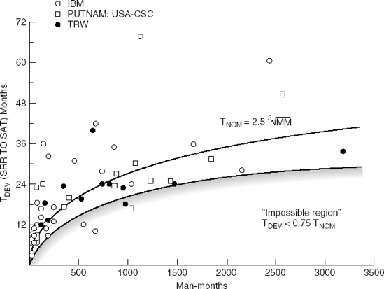
Everything takes time. We can not shorten a software development project indefinitely by trading off time against people. Boehm sets the limit at 75% of the nominal development time, on empirical grounds. A system that has to be delivered too fast gets into the 'impossible region' (see Figure 7.3). The chance of success becomes almost nil if the schedule is pressed too far.
In any case, a shorter development time induces higher costs. We may use the following rule of thumb: compressing the development time by X% results in a cost increase of X% relative to the nominal cost estimate (Boehm, 1984a).
One of the key values of agile development is that one should respond to change rather than follow a plan. This key value translates to a different attitude towards cost estimation as well. In agile development, there is no cost estimation for the whole project in advance. Since we assume things will change, such an upfront, overall cost estimation is considered useless. Usually, an agile development project delivers functionality in a number of iterations. Each iteration provides the user with a number of features. The number of features may be fixed and the next version is released when all features agreed upon have been implemented. Alternatively, the release date may be fixed and then the number of features is adjusted to fit the time box.
In either case, we are interested in estimating the cost and duration of a set of features. Doing this the agile way, the cost estimation proceeds in two steps:
Estimate the effort on a scale which is unitless.
Translate the effort estimation into a duration.
In Step 1, the effort required for each feature is estimated relative to the effort estimated for the other features. The unit in which the effort is expressed has no relation to actual time. Cohn (2006) calls them story points. One way to estimate the story points for a set of features is to first look for a feature that you think will require average effort. This feature, A, is assigned an average number of story points, say 5. Next, the other features are estimated relative to A. If you think feature B requires about half the effort of feature A, it is assigned 2 (or 3) story points. If B is estimated to require twice the effort of A, it is assigned ten story points. And so on, until all features have been assigned a story point size.
This process works best if the size of the features differs by at most one order of magnitude. It is difficult to accurately estimate the effort of a set of features if, say, some require 2 story points, while others require 100. One easy way to assign story points is to only use the values 1, 2, 4 and 8, say. A feature is then estimated to be double or half the size of another feature. Very small features may be estimated at 0 story points. Of course, you can't have too many features of size 0.
Agile development is a team effort and so is agile estimation. All team members may be involved in the estimation process. Cohn (2006) describes a poker-like game for doing this. For a given feature, all participants individually estimate the number of story points required and write their estimate on a card. All the cards are turned over at the same time. If you're lucky, the numbers on the cards are approximately the same. If the numbers vary widely, the participants explain why they estimated the effort the way they did. Once these explanations have been given, the poker game for that feature is repeated. Hopefully, the variation in the effort estimates will decrease. The process is repeated until the estimates are sufficiently similar. Note that this process is more than an entertaining estimation exercise. While explaining their estimates, tacit knowledge about the feature and its possible implementation is shared. The group effectively does part of the design while estimating.
After the effort for each feature has been estimated, the actual time needed per effort point is estimated. This is done by estimating the velocity. The velocity is the number of story points completed in one iteration. It is a measure of progress. For instance, the team might estimate it can implement eight story points in two weeks. This estimate is based on the team's experience with earlier projects. In maintenance, similar lines of thought are used when estimating the probability that components require changes, based on the change history of those components. It is commonly referred to as yesterday's weather: without any additional knowledge, we assume today's weather will be like yesterday's. As the project progresses, the team will accumulate knowledge about its performance and will estimate its velocity more accurately.
If the team does not manage to implement as many story points as it hoped to implement during the iteration, there is no immediate need to adjust the story points of features. Story points should only be adjusted if the relative size of a feature changes. The only thing that matters is that they are mutually consistent. If the schedule does not fit, it is more likely that the team overestimated the number of story points it can realize in a week.
Story points are a valid measure of effort only for the current project and the current team. Just as algorithmic models need to be calibrated for each organization, story points need to be determined anew for a new situation. For example, a feature that is estimated at 4 story points in one situation, may well be estimated at 8 story points in another. After all, it is an effort estimate relative to the effort required for the other features. If the other features change, so will the estimate. In the same vein, the velocity depends on the current project and the current team. In one project, a story point may amount to one week of work, while in another project a story point may take a month. A less experienced team might take two months for that same story point.
Story points are a pure measure of size. They only measure the size of features relative to one another. They have nothing to do with 'real' working days. People outside the team may have difficulty coping with the abstract nature of story points. As an alternative to story points, Cohn (2006) suggests using ideal days. An ideal day is a day in which you can work uninterrupted on a single feature. There are no phone calls from the customer, no meetings, no questions from the help desk that need an answer, no time lost because you are working on two things at the same time, etc. Similarly to the step from story points to real speed, in a second step the ideal days are translated into real days, taking into account all the factors that slow people down.
It remains to be seen whether we will ever get one general cost estimation model. The number of parameters that impact productivity simply seems to be too large. Yet, each organization may develop a model which is well suited for projects to be undertaken within that organization. An organization may, and should, build a database with data on its own projects. Starting with a model such as COCOMO 2, the different parameters, i.e. applicable cost drivers and values for the associated effort multipliers, may then be determined. In the course of time, the model becomes more closely tuned to the organizational environment, resulting in better and better estimates. Reifer (2000), for example, describes how COCOMO 2 can be adapted to estimate for Web-based software development projects.
A word of caution: present-day algorithmic cost models are not all that good yet. At best, they yield estimates which are at most 25% off, 75% of the time, for projects used to derive the model. Expert-based cost estimates and the much simpler models that are based on counting a fairly small number of attributes, use-case points, or story points are a viable alternative.
Even when much better performance is realized, some problems remain when using the type of cost estimation model obtained in this way:
Even though a model such as COCOMO 2 looks objective, a fair amount of subjectivity is introduced through the need to assign values to the various levels of a number of cost drivers. Based on an analysis of historical project data, Jones (1986) lists 20 factors which certainly influence productivity and another 25 for which it is probable. The set of COCOMO 2 cost drivers already allows for a variation of 1:800. A much smaller number of relevant cost drivers would reduce a model's vulnerability to the subjective assessment of project characteristics.
The models are based on data from old projects and reflect the technology of those projects. In some cases, the project data may be quite old. The impact of more recent developments cannot easily be taken into account, since we do not have sufficient data on projects which exhibit those characteristics.
Almost all models take into account attributes that impact the initial development of software. Attributes which specifically relate to maintenance activities are seldom taken into account. Also, factors such as the amount of documentation required or the number of business trips (in the case of a multi-site development) are often lacking. Yet, these factors may have a significant impact on the effort needed.
Algorithmic models usually result from applying statistical techniques such as regression analysis to a given set of project data. For a new project, the parameters of the model have to be determined and the model yields an estimate and, in some cases, a confidence interval.
In the introduction to this chapter, we compared cost estimation for software development with cost estimation for laying out a garden. When laying out a garden, we often follow a rather different line of thought, namely: given a budget of, say, $10 000, what possibilities are there? What happens if we trade off a pond against something else? Something similar is also possible with software. Given a budget of $100 000 for library automation, what possibilities are there? Which user interface can we expect? What will the transaction speed be? How reliable will the system be? To be able to answer these types of question, we need to be able to analyze the sensitivity of an estimate to varying values of relevant attributes.
Finally, estimating the cost of a software development project is a highly dynamic activity. Not only may we switch from one model to another during the course of a project, estimates are also adjusted on the basis of experiences gained. Switching to another model during the execution of a project is possible, since we may expect to get more reliable data while the project is making progress. We may, for instance, imagine using the series of increasingly detailed COCOMO 2 models. When using some agile estimation approach, the estimates will improve over time as knowledge about one's performance increases.
We cannot, and should not, rely on a one-shot cost estimate. Controlling a software development project implies a regular check of progress, a regular check of estimates made, re-establishing priorities and weighing stakes, as the project progresses.
Early cost estimation models are described in (Nelson, 1966) and (Wolverton, 1974). The Walston–Felix model is described in (Walston and Felix, 1977). The model of Putnam and Norden is described in (Norden, 1970) and (Putnam, 1978). Boehm (1981) is the definitive source on the original COCOMO model. COCOMO 2 is described in (Boehm et al., 1997) and (Boehm et al., 2000).
Function point analysis (FPA) is developed by (Albrecht, 1979) and (Albrecht and Gaffney, 1983). Critical appraisals of FPA can be found in (Symons, 1988), (Kemerer, 1993), (Kemerer and Porter, 1992), (Abran and Robillard, 1992) and (Abran and Robillard, 1996). A detailed discussion of function points, its counting process and some case studies, is provided by (Garmus and Herron, 1996). (Costagliola et al., 2005) describe a function-point type measure for object-oriented systems. Use case points were introduced in (Karner, 1993). Experiences with use case points are described in (Carroll, 2005) and (Mohagheghi et al., 2005).
Cohn (2006) is a very good book on agile estimation. McConnell (2006) is a more general book on effort estimation.
The relation between project behavior and its cost estimate is discussed in (Abdel-Hamid et al., 1993). Guidelines for cost estimation are given in (Boehm and Sullivan, 1999), (Fairley, 2002) and (Jørgensen, 2005). Jørgensen (2004) gives an overview of studies on expert estimation. Jørgensen (2005) gives useful guidelines for expert-based effort estimation. (Software, 2000) is a special issue devoted to software estimation.
In which ways may political arguments influence cost estimates?
What does the Walston–Felix model look like?
How may the Rayleigh curve be related to software cost estimation?
Give a sketch of function point analysis (FPA).
Give a sketch of COCOMO 2.
Discuss the major differences between COCOMO 2 and FPA.
Give a rationale for Brooks' Law.
In which sense does function point analysis (FPA) reflect the batch-oriented world of the 1970s?
How may early cost estimates influence the way in which a project is executed?
Why is it difficult to compare different cost estimation models?
Discuss how to estimate feature size using story points.
Explain the cone of uncertainty.
Suppose you are involved in a project which is estimated to take 100 man-months. How would you estimate the nominal calendar time required for this project? Suppose the project is to be finished within six calendar months. Do you think such a schedule compression is feasible?
Why should software cost models be recalibrated from time to time?

