
LEARNING OBJECTIVES
To be able to discern desirable properties of a software design
To understand different notions of complexity, at both the component and system level
To be aware of some object-oriented metrics
To be aware of some widely known classical design methods
To understand the general flavor of object-oriented analysis and design methods
To be aware of a global classification scheme for design methods
To understand the role of design patterns and be able to illustrate their properties
To be aware of guidelines for the design documentation
Note
Software design concerns the decomposition of a system into its constituent parts. A good design is the key to the successful implementation and evolution of a system. A number of guiding principles for this decomposition help to achieve quality designs. These guiding principles underlie the main design methods discussed in this chapter. Unlike more classical design fields, there is no visual link between the design representation of a software system and the ultimate product. This complicates the communication of design knowledge and raises the importance of proper design representations.
During software development, we should adhere to a planned approach. If we want to travel from point A to point B, we will (probably) consult a map first. According to some criterion, we will then plan our route. The time-loss caused by the planning activity is bound to outweigh the misery that occurs if we do not plan our trip at all but just take the first turn left, hoping that this will bring us somewhat closer to our destination. In designing a garden, we also follow some plan. We do not start by planting a few bulbs in one corner, an apple tree in another, and a poplar next to the front door.
The above examples sound ridiculous. They are. Yet, many a software development project is undertaken in this way. Somewhat exaggeratedly, we may call it the 'programmer's approach' to software development. Much software is still being developed without a clear design phase. The reasons for this 'code first, design later' attitude are many:
We do not want to, or are not allowed to, 'waste our time' on design activities.
We have to, or want to, quickly show something to our customer.
We are judged by the amount of code written per man-month.
We are, or expect to be, pressed for time.
For many types of system (just think of an airline reservation system), such an approach grossly underestimates the complexity of software and its development. Just as with the furnishing of a house or the undertaking of a long trip, it is paramount to put thought into a plan, resulting in a blueprint that is then followed during actual construction. The outcome of this process (the blueprint) will be termed the design or, if the emphasis is on its notation, the (technical) specification. The process of making this blueprint is also called design. To a large extent, the quality of the design determines the quality of the resulting product. Errors made during the design phase often go undetected until the system is operational. At that time, they can be repaired only by incurring very high costs.
Software design is a 'wicked problem'. The term originated in research into the nature of design issues in social planning problems. Properties of wicked problems in this area are remarkably similar to properties of software design:
A wicked problem has no definite formulation. The design process can hardly be separated from either the preceding requirements engineering phase or the subsequent documentation of the design in a specification. These activities will, in practice, overlap and influence each other. At the more global (architectural) stages of system design, the designer will interact with the user to assess fitness-for-use aspects of the design. This may lead to adaptations in the requirements specification. The more detailed stages of design often cannot be separated from the specification method used. One corollary of this is that the waterfall model does not fit the type of problem it is meant to address.
A wicked problem has no stopping rule. There is no criterion that tells us when the solution has been reached. Though we do have a number of quality measures for software designs, there does not exist a single scale against which to measure the quality of a design. There probably never will be such a scale.
The solution to a wicked problem is not true or false. At best, it is good or bad. The software design process is not analytic. It does not consist of a sequence of decisions each of which brings us somewhat closer to that one, optimal solution. Software design involves making a large number of tradeoffs, such as those between speed and robustness. As a consequence, there is a number of acceptable solutions, rather than one best solution.
Every wicked problem is a symptom of another problem. Resolving one problem may very well result in an entirely different problem elsewhere. For example, the choice of a particular dynamic data structure may solve the problem of an unknown input size and at the same time introduce an efficiency problem. A corollary of this is that small changes in requirements may have large consequences in the design or implementation. In Chapter 1, we described this by saying that software is not continuous.
During design we may opt for a Taylorian, functionality-centered view and consider the design problem as a purely technical issue. Alternatively, we may realize that design involves user issues as well and therefore needs some form of user involvement. The role of the user during design need not be restricted to that of a guinea-pig in shaping the actual user interface. It may also involve much deeper issues.
Rather than approaching system design from the point of view that human weaknesses need to be compensated for, we may take a different stand and consider computerized systems as a way of supporting human strengths. Likewise, systems need not reflect the interests of system owners only. In a democratic world, systems can be designed so that all those involved benefit. This less technocratic attitude leads to extensive user involvement during all stages of system development. Agile development methods advocate this type of approach.
Whereas traditional system development has a production view in which the technical aspects are optimized, the 'Scandinavian school' pays equal attention to the human system and holds the view that technology must be compatible with organizational and social needs. The various possible modes of interaction between the designer or analyst on the one hand and the user on the other hand are also discussed in Section 9.1.
Pure agile approaches do suggest starting by planting just a few bulbs in one corner of the garden. If we happen to move into our new house in late fall and want some color when spring sets in, this sounds like the best thing we can do. If we change our mind at some later point in time, we can always move the bulbs and do some additional garden design. It thus depends on the situation at hand how much upfront design is feasible (see also Chapter 8). In this chapter, we assume enough context and requirements are known to warrant an explicit design step. Of course, there may be successive design steps in successive iterations.
From the technical point of view, the design problem can be formulated as follows: how can we decompose a system into parts such that each part has a lower complexity than the system as a whole, while the parts together solve the user's problem? Since the complexity of the individual components should be reasonable, it is important that the interaction between components is not too complicated.
Design has both a product aspect and a process aspect. The product aspect refers to the result, while the process aspect is about how we get there. At the very global, architectural levels of design, there is little process guidance, and the result is very much determined by the experience of the designer. For that reason, Chapter 11 largely focuses on the characterization of the result of the global design process, the software architecture. In this chapter, we focus on the more detailed stages of design, where more process guidance has been accumulated in a number of software design methods. But for the more detailed stages of software design too, the representational aspect is the more important one. This representation is the main communication vehicle between the designer and the other stakeholders. Unlike more classical design fields, there is no visual link between the design representations of a software system and the ultimate product. The blueprint of a bridge gives us lots of visual clues as to how that bridge will eventually look. This is not the case for software and we have to seek other ways to communicate design knowledge to our stakeholders.
There really is no universal design method. The design process is a creative one, and the quality and expertise of the designers are a critical determinant for its success. However, over the years a number of ideas and guidelines have emerged which may serve us in designing software.
The single most important principle of software design is information hiding. It exemplifies how to apply abstraction in software design. Abstraction means that we concentrate on the essential issues and ignore, abstract from, details that are irrelevant at this stage. Considering the complexity of the problems we are to solve, applying some sort of abstraction is a sheer necessity. It is simply impossible to take in all the details at once.
Section 12.1 discusses desirable design properties that bear on quality issues, most notably maintainability and reusability. Five properties are identified that have a strong impact on the quality of a design: abstraction, modularity, information hiding, complexity, and system structure. Assessment of a design with respect to these properties allows us to get an impression of design quality, albeit not a very quantitative one yet. Efforts to quantify such heuristics have resulted in a number of metrics specifically aimed at object-oriented systems.
A vast number of design methods exist, many of which are strongly tied to a certain notation. These methods give strategies and heuristics to guide the design process. Most methods use a graphical notation to depict the design. Though the details of those methods and notations differ widely, it is possible to provide broad characterizations in a few classes. The essential characteristics of those classes are elaborated upon in Sections 12.2 and 12.3.
Design patterns are collections of a few components (or, in object-oriented circles, classes) which are often used in combination and which together provide a useful abstraction. A design pattern is a recurring solution to a standard problem. The opposite of a pattern is an antipattern: a mistake often made. The prototypical example of a pattern is the Model-View-Controller (MVC) pattern from Smalltalk. A well-known antipattern is the Swiss Army Knife: an overly complex class interface. Design patterns and antipatterns are discussed in Section 12.5.
During the design process, quite a lot of documentation is generated. This documentation serves various users, such as project managers, designers, testers, and programmers. Section 12.6 discusses IEEE Standard 1016. This standard contains useful guidelines for describing software designs. The standard identifies a number of roles and indicates, for each role, the type of design documentation needed.
Finally, Section 12.7 discusses some verification and validation techniques that may fruitfully be applied at the design stage.
Up till now we have used the notion of 'component' in a rather intuitive way. It is not easy to give an accurate definition of that notion. Obviously, a component does not denote some random piece of software. We apply certain criteria when decomposing a system into components.
At the programming-language level, a component usually refers to an identifiable unit with respect to compilation. We will use a similar definition of the term 'component' with respect to design: a component is an identifiable unit in the design. It may consist of a single method, a class, or even a set of classes. It preferably has a clean interface to the outside world and the functionality of the component then is only approached through that interface.
There are, in principle, many ways to decompose a system into components. Obviously, not every decomposition is equally desirable. In this section, we are interested in desirable properties of a decomposition, irrespective of the type of system or the design method used. These properties can in some sense be used as a measure of the quality of the design. Designs that have those properties are considered superior to those that do not have them.
The design properties we are most interested in are those that facilitate maintenance and reuse: simplicity, a clear separation of concepts into different components, and restricted visibility (i.e. locality) of information.[14] Systems that have those properties are easier to maintain since we may concentrate our attention on those parts that are directly affected by a change. These properties also bear on reusability, because the resulting components tend to have a well-defined functionality that fits concepts from the application domain. Such components are likely candidates for inclusion in other systems that address problems from the same domain.
In the following subsections, we discuss five interrelated issues that have a strong impact on the above properties:
For object-oriented systems, a specific set of quality heuristics and associated metrics has been defined. The main object-oriented metrics are discussed in Section 12.1.6.
Abstraction means that we concentrate on the essential properties and ignore, abstract from, details that are not relevant at the level we are currently working. Consider, for example, a typical sorting component. From the outside we cannot (and need not be able to) discern exactly how the sorting process takes place. We need only know that the output is indeed sorted. At a later stage, when the details of the sorting component are decided upon, then we can rack our brains about the most suitable sorting algorithm.
The complexity of most software problems makes applying abstraction a sheer necessity. In the ensuing discussion, we distinguish two types of abstraction: procedural abstraction and data abstraction.
The notion of procedural abstraction is fairly traditional. A programming language offers if constructs, loop constructs, assignment statements, and so on. The transition from a problem to be solved to these primitive language constructs is a large one in many cases. To this end, a problem is first decomposed into subproblems, each of which is handled in turn. These subproblems correspond to major tasks to be accomplished. They can be recognized by their description, in which some verb plays a central role (for example, read the input, sort all records, process the next user request, compute the net salary). If needed, subproblems are further decomposed into even simpler subproblems. Eventually we get at subproblems for which a standard solution is available. This type of (top-down) decomposition is the essence of the main-program-with-subroutines architectural style (see Section 11.4).
The result of this type of stepwise decomposition is a hierarchical structure. The top node of the structure denotes the problem to be solved. The next level shows its first decomposition into subproblems. The leaf nodes denote primitive problems. This is schematically depicted in Figure 12.1.
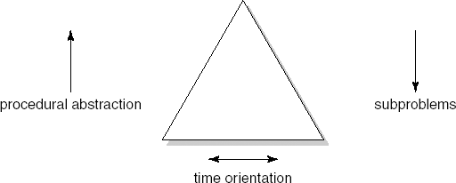
The procedure concept offers us a notation for the subproblems that result from this decomposition process. The application of this concept is known as procedural abstraction. With procedural abstraction, the name of a procedure (or method, in object-oriented languages) is used to denote the corresponding sequence of actions. When that name is used, we need not bother ourselves about the exact way in which its effect is realized. The important thing is that, after the call, certain prestated requirements are fulfilled.
This way of going about the process closely matches the way in which humans are inclined to solve problems. Humans too are inclined to the stepwise handling of problems. Procedural abstraction thus offers an important means of tackling software problems.
When designing software, we are inclined to decompose the problem so that the result has a strong time orientation. A problem is decomposed into subproblems that follow each other in time. In its simplest form, this approach results in input – process – output schemes: a program first has to read and store its data, next some process computes the required output from this data, and the result finally is output. Application of this technique may result in programs that are difficult to adapt and hard to comprehend. Applying data abstraction results in a decomposition which shows this affliction to a far lesser degree.
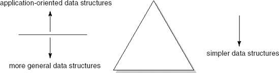
Procedural abstraction is aimed at finding a hierarchy in the program's control structure: which steps have to be executed and in which order. Data abstraction is aimed at finding a hierarchy in the program's data. Programming languages offer primitive data structures for integers, real numbers, truth values, characters and possibly a few more. Using these building blocks, we may construct more complicated data structures, such as stacks and binary trees. Such structures are of general use in application software. They occur at a fairly low level in the hierarchy of data structures. Application-oriented objects, such as 'paragraph' in text-processing software or 'book' in our library system, are found at higher levels of the data structure hierarchy. This is schematically depicted in Figure 12.2.
For the data, too, we wish to abstract from details that are not relevant at a certain level. In fact, we already do so when using the primitive data structures offered by our programming language. In using these, we abstract from details such as the internal representation of numbers and the way in which the addition of two numbers is realized. At the programming language level we may view the integers as a set of objects (0, 1, −1, 2, −2, ...) and a set of operations on these objects (+, −, ×, /, ...). These two sets together determine the data type integer. To be able to use this data type, we need only name the set of objects and specify its operations.
We may proceed along the same lines for the data structures not directly supported by the programming language. A data type binary-tree is characterized by a set of objects (all conceivable binary trees) and a set of operations on those objects. When using binary trees, their representation and the implementation of the corresponding operations need not concern us. We need only ascertain the intended effect of the operations.
Applying data abstraction during design is sometimes called object-oriented design, since the type of object and the associated operations are encapsulated in one component. The buzzword 'object-oriented' however also has a subtly different meaning in the context of design. We will further elaborate upon this notion in Section 12.3.
Languages such as Ada, Java and C++ offer a language construct (called package, class, and struct, respectively) that allows us to maintain a syntactic separation between the implementation and specification of data types. Note that it is also possible to apply data abstraction during design when the ultimate language does not offer the concept. However, it then becomes more cumbersome to move from design to code.
We noticed before that procedural abstraction fits in nicely with the way humans tend to tackle problems. To most people, data abstraction is a bit more complicated.
When searching for a solution to a software problem we will find that the solution needs certain data structures. At some point we will also have to choose a representation for these data structures. Rather than making those decisions at an early stage and imposing the result on all other components, you are better off if you create a separate subproblem and make only the procedural, implementation-independent, interfaces public. Data abstraction thus is a prime example of information hiding.
The development of these abstraction techniques went hand-in-hand with other developments, particularly those in the realm of programming languages. Procedures were originally introduced to avoid the repetition of sequences of instructions. At a later stage, we viewed the name of a procedure as an abstraction of the corresponding instruction sequence. Only then did the notion of procedural abstraction get its present connotation. In a similar vein, developments in the field of formal data type specifications and language notions for components (starting with the class concept of SIMULA-67) strongly contributed to our present notion of data abstraction.
As a final note, we remark that we may identify yet a third type of abstraction, control abstraction. In control abstraction, we abstract from the precise order in which a sequence of events is to be handled. Though control abstraction is often implicit when procedural abstraction is used, it is sometimes convenient to be able to explicitly model this type of nondeterminacy, for instance when specifying concurrent systems. This topic falls outside the scope of this book.
During design, the system is decomposed into a number of components and the relationships between those components are indicated. In another design of the same system, different components may show up and there may be different relationships between the components. We may try to compare those designs by considering both a typology for the individual components and the type of connections between them. This leads us to two structural design criteria: cohesion and coupling.
Cohesion may be viewed as the glue that keeps the component together. It is a measure of the mutual affinity of the elements of a component. In general we will wish to make the cohesion as strong as possible. In their classic text, Yourdon and Con-stantine (1975) identify the following seven levels of cohesion of increasing strength:
Coincidental cohesion: Elements are grouped into components in a haphazard way. There is no significant relation between the elements.
Logical cohesion: Elements realize tasks that are logically related. One example is a component that contains all input routines. These routines do not call one another and they do not pass information to each other. Their function is just very similar.
Temporal cohesion: The elements are independent but they are activated at about the same point in time. A typical example of this type of cohesion is an initialization component.
Procedural cohesion: The elements have to be executed in a given order. For instance, a component may have to first read some data, then search a table, and finally print a result.
Communicational cohesion: The elements of a component operate on the same (external) data. For instance, a component may read some data from a disk, perform certain computations on the data, and print the result.
Sequential cohesion: The component consists of a sequence of elements where the output of one element serves as input to the next element.
Functional cohesion: All elements contribute to a single function. Such a component often transforms a single input into a single output. The well-known mathematical subroutines are a typical example of this. Less trivial examples are components such as 'execute the next edit command' and 'translate the program given'.
In a classic paper on structured design, (Stevens et al., 1974) provide some simple heuristics that may be of help in establishing the degree of cohesion of a component. They suggest writing down a sentence that describes the function (purpose) of the component and examining that sentence. Properties to look for include the following:
If the sentence is compound, has a connective (such as a comma or the word 'and'), or contains more than one verb, then that component is probably performing more than one function. It is likely to have sequential or communicational cohesion.
If the sentence contains words that relate to time (such as 'first', 'next', 'after', and 'then'), then the component probably has sequential or temporal cohesion.
If the sentence contains words such as 'initialize', the component probably has temporal cohesion.
The levels of cohesion identified above reflect the cohesion between the functions that a component provides. Abstract data types cannot easily be accommodated in this scheme. Macro and Buxton (1987) therefore propose adding an extra level, data cohesion, to identify components that encapsulate an abstract data type. Data cohesion is even stronger than functional cohesion.
It goes without saying that it is not always an easy task to obtain the strongest possible cohesion between the elements of a component. Though functional cohesion may be attainable at the top levels and data cohesion at the bottom levels, we often have to settle for less at the intermediate levels of the component hierarchy. The tradeoffs to be made here are what makes design such a difficult, and yet challenging, activity.
The second structural criterion is coupling. Coupling is a measure of the strength of the intercomponent connections. A high degree of coupling indicates a strong dependence between components. A high degree of coupling between components means that we can only fully comprehend this set of components as a whole and may result in ripple effects when a component has to be changed, because such a change is likely to incur changes in the dependent components as well. Loosely coupled components, on the other hand, are relatively independent and are easier to comprehend and adapt. Loose coupling therefore is a desirable property of a design (and its subsequent realization). The following types of coupling can be identified (from tightest to loosest):
Content coupling: One component directly affects the working of another component. Content coupling occurs when a component changes another component's data or when control is passed from one component to the middle of another (as in a jump). This type of coupling can, and should, always be avoided.
Common coupling: Two components have shared data. The name originates from the use of COMMON blocks in FORTRAN. Its equivalent in block-structured languages is the use of global variables.
External coupling: Components communicate through an external medium, such as a file.
Control coupling: One component directs the execution of another component by passing the necessary control information. This is usually accomplished by means of flags that are set by one component and reacted upon by the dependent component.
Stamp coupling: Complete data structures are passed from one component to another. With stamp coupling, the precise format of the data structures is a common property of those components.
Data coupling: Only simple data is passed between components.
The various types of coupling emerged in the 1970s and reflect the data type concepts of programming languages in use at that time. For example, programming languages of that time had simple scalar data types such as real and integer. They allowed arrays of scalar values and records were used to store values of different types. Components were considered data-coupled if they passed scalars or arrays. They were considered stamp-coupled if they passed record data. When two components are control-coupled, the assumption is that the control is passed through a scalar value.
Nowadays, programming languages have much more flexible means of passing information from one component to another, and this requires a more detailed set of coupling levels. For example, components may pass control data through records (as opposed to scalars only). Components may allow some components access to their data and deny it to others. As a result, there are many levels of visibility. The coupling between components need not be commutative. When component A passes a scalar value to B and B returns a value which is used to control the further execution of A, then A is data-coupled to B, while B is control-coupled to A. As a result, people have extended and refined the definitions of cohesion and coupling levels.
Coupling and cohesion are dual characteristics. If the various components exhibit strong internal cohesion, the intercomponent coupling tends to be minimal, and vice versa.
Simple interfaces — weak coupling between components and strong cohesion among a component's elements — are of crucial importance for a variety of reasons:
Communication between programmers becomes simpler. When different people are working on the same system, it helps if decisions can be made locally and do not interfere with the working of other components.
Correctness proofs become easier to derive.
It is less likely that changes will propagate to other components, which reduces maintenance costs.
The reusability of components is increased. The fewer assumptions that are made about an element's environment, the greater the chance of fitting another environment.
The comprehensibility of components is increased. Humans have limited memory capacity for information processing. Simple component interfaces allow for an understanding of a component independent of the context in which it is used.
Empirical studies show that interfaces exhibiting weak coupling and strong cohesion are less error-prone than those that do not have these properties.
The concept of information hiding originates from a seminal paper (Parnas, 1972). The principle of information hiding is that each component has a secret which it hides from other components.
Design involves a sequence of decisions, such as how to represent certain information, or in which order to accomplish tasks. For each such decision we should ask ourselves which other parts of the system need to know about the decision and how it should be hidden from parts that do not need to know.
Information hiding is closely related to the notions of abstraction, cohesion, and coupling. If a component hides some design decision, the user of that component may abstract from (ignore) the outcome of that decision. Since the outcome is hidden, it cannot possibly interfere with the use of that component. If a component hides some secret, that secret does not penetrate the component's boundary, thereby decreasing the coupling between that component and its environment. Information hiding increases cohesion, since the component's secret is what binds the component's constituents together. Note that, in order to maximize its cohesion, a component should hide one secret only.
It depends on the programming language used whether the separation of concerns obtained during the design stage will be identifiable in the ultimate code. To some extent, this is of secondary concern. The design decomposition will be reflected, if only implicitly, in the code and should be explicitly recorded (for traceability purposes) in the technical documentation. It is of great importance for the later evolution of the system. A confirmation of the impact of such techniques as information hiding on the maintainability of software can be found in (Boehm, 1983).
Like all good inventions, readability yardsticks can cause harm in misuse. They are handy statistical tools to measure complexity in prose. They are useful to determine whether writing is gauged to its audience. But they are not formulae for writing. ... Writing remains an art governed by many principles. By no means all factors that create interest and affect clarity can be measured objectively.
Gunning (1968)
In a very general sense, the complexity of a problem refers to the amount of resources required for its solution. We may try to determine complexity in this way by measuring, say, the time needed to solve a problem. This is called an external attribute: we are not looking at the entity itself (the problem), but at how it behaves.
In the present context, complexity refers to attributes of the software that affect the effort needed to construct or change a piece of software. These are internal attributes: they can be measured purely in terms of the software itself. For example, we need not execute the software to determine their values.
Both these notions are very different from the complexity of the computation performed (with respect to time or memory needed). The latter is a well-established field in which many results have been obtained. This is much less true for the type of complexity in which we are interested. Software complexity in this sense is still a rather elusive notion.
Serious efforts have been made to measure software complexity in quantitative terms. The resulting metrics are intended to be used as anchor points for the decomposition of a system, to assess the quality of a design or program, to guide reengineering efforts, etc. We then measure certain attributes of a software system, such as its length, the number of if statements, or the information flow between components, and try to relate the numbers thus obtained to the system's complexity. The type of software attributes considered can be broadly categorized into two classes:
intracomponent attributes are attributes of individual components, and
intercomponent attributes are attributes of a system viewed as a collection of components with dependencies.
In this subsection, we are dealing with intracomponent attributes. Intercompo-nent attributes are discussed in Section 12.1.5. We may distinguish two classes of complexity metrics:
Size-based complexity metrics. The size of a piece of software, such as the number of lines of code, is fairly easy to measure. It also gives a fair indication of the effort needed to develop that piece of software (see also Chapter 7). As a consequence, it could also be used as a complexity metric.
Structure-based complexity metrics. The structure of a piece of software is a good indicator of its design quality, because a program that has a complicated control structure or uses complicated data structures is likely to be difficult to comprehend and maintain, and thus more complex.
The easiest way to measure software size is to count the number of lines of code. We may then impose limits on the number of lines of code per component. In (Weinberg, 1971), for instance, the ideal size of a component is said to be 30 lines of code. In a variant, limits are imposed on the number of elements per component. Some people claim that a component should contain at most seven elements. This number seven can be traced back to research in psychology, which suggests that human memory is hierarchically organized with a short-term memory of about seven slots, while there is a more permanent memory of almost unlimited capacity. If there are more than seven pieces of information, they cannot all be stored in short-term memory and information gets lost.
There are serious objections to the direct use of the number of lines of code as a complexity metric. Some programmers write more verbose programs than others. We should at least normalize the counting to counteract these effects and be able to compare different pieces of software.
A second objection is that this technique makes it hard to compare programs written in different languages. If the same problem is solved in different languages, the results may differ considerably in length. For example, APL is more compact than COBOL.
Finally, some lines are more complex than others. An assignment statement such as:
a = b
looks simpler than a loop:
while (current = null) {current = current.next;}although they each occupy one line.
Halstead (1977) uses a refinement of counting lines of code. This refinement is meant to overcome the problems associated with metrics based on a direct count of lines of code.
Halstead's method, also known as 'software science', uses the number of operators and operands in a piece of software. The set of operators includes the arithmetic and Boolean operators, as well as separators (such as a semicolon between adjacent instructions) and (pairs of) reserved words. The set of operands contains the variables and constants used. Halstead then defines four basic entities:
n1 is the number of unique (i.e. different) operators in the component;
n2 is the number of unique (i.e. different) operands in the component;
N1 is the total number of occurrences of operators;
N2 is the total number of occurrences of operands.
Figure 12.3 contains a simple sorting routine. Table 12.1 lists the operators and operands of this routine together with their frequencies. Note that there is no generally agreed definition of what exactly an operator or operand is, so the numbers given have no absolute meaning. This is part of the criticism of this theory.
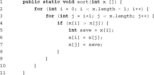
Table 12.1. Counting the number of operators and operands in the sort routine
Operator | Number of occurrences | Operand | Number of occurrences |
|---|---|---|---|
| 1 |
| 9 |
| 1 |
| 2 |
| 1 |
| 7 |
| 1 |
| 6 |
| 4 |
| 2 |
| 7 |
| 1 |
{ } | 4 |
| 2 |
| 2 | ||
| 5 | ||
< | 2 | ||
| 2 | ||
| 1 | ||
| 2 | ||
| 1 | ||
| 1 | ||
> | 1 | ||
| 3 | ||
n1 = 17 | N1 = 39 | n2 = 7 | N2 = 29 |
Using the primitive entities defined above, Halstead defines a number of derived entities, such as:
Size of the vocabulary: n = n1 + n2.
Program length: N = N1 + N2.
Program volume: V = N log 2 n.
This is the minimal number of bits needed to store N elements from a set of cardinality n.
Program level: L = V*/V.
Here V* is the most compact representation of the algorithm in question. For the example in Figure 12.3 this is
sort(x);, so n = N = 3, and V* = 3 log 2 3. From the formula, it follows that L is at most 1. Halstead postulates that the program level increases if the number of different operands increases, while it decreases if the number of different operators or the total number of operands increases. As an approximation of L, he therefore suggests:
Programming effort: E = V/L.
The effort needed increases with volume and decreases as the program level increases. E represents the number of mental discriminations (decisions) to be taken while implementing the problem solution.
Estimated programming time in seconds:

The constant 18 is determined empirically. Halstead explains this number by referring to (Stroud, 1967), which discusses the speed with which human memory processes sensory input. This speed is said to be 5–20 units per second. In Halstead's theory, the number 18 is chosen. This number is also referred to as Stroud's number.
The above entities can only be determined after the program has been written. It is, however, possible to estimate a number of these entities. When doing so, the values for n1 and n2 are assumed to be known. This may be the case, for instance, after the detailed design step. Halstead then estimates program length as:
An explanation for this formula can be given as follows. There are n12n1 × n22n2 ways to combine the n given symbols such that operators and operands alternate. However, the program is organized and organization generally gives a logarithmic reduction in the number of possibilities. Doing so yields the above formula for
Table 12.2. Values for 'software science' entities for the routine in Figure 12.3
Entity | Value |
|---|---|
Size vocabulary | 24 |
Program length | 68 |
Estimated program length | 89 |
Program volume | 312 |
Level of abstraction | 0.015 |
Estimated level of abstraction | 0.028 |
Programming effort | 20 800 |
Estimated programming time | 1 155 |
A number of empirical studies have addressed the predictive value of Halstead's formulae. These studies often give positive evidence of the validity of the theory.
The theory has also been heavily criticized. The underpinning of Halstead's formulae is not convincing. Results from cognitive psychology, such as Stroud's number, are badly used, which weakens the theoretical foundation. Halstead concentrates on the coding phase and assumes that programmers are 100% devoted to a programming task for an uninterrupted period of time. Practice is likely to be quite different. Different people use quite different definitions of the notions of operator and operand, which may lead to widely different outcomes for the values of entities. Yet, Halstead's work has been very influential. It was the first major body of work to point out the potential of metrics for software development.
The second class of intracomponent complexity metrics concerns metrics based on the structure of the software. If we try to derive a complexity metric from the structure of a piece of software, we may focus on the control structure, the data structures, or a combination of these.
If we base the complexity metric on the use of data structures, we may do so by considering, for instance, the number of instructions between successive references to one object. If this number is large, information about these variables must be retained for a long period of time when we try to comprehend that program text. Following this line of thought, complexity can be related to the average number of variables for which information must be kept by the reader.
The best-known structure-based complexity metric is McCabe's cyclomatic complexity (McCabe, 1976). McCabe bases his complexity metric on a (directed) graph depicting the control flow of a component. He assumes that the graph of a single component has a unique start and end node, that each node is reachable from the start node, and that the end node can be reached from each node. In that case, the graph is connected. If the component is a class consisting of one or more methods, then the control graph has a number of connected subgraphs, one for each of its methods.
The cyclomatic complexity, CV, equals the number of predicates (decisions) plus 1 in the component that corresponds to this control graph. Its formula reads
where e, n and p denote the number of edges, nodes, and connected subgraphs in the control graph, respectively.
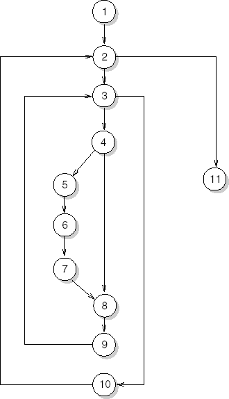
Figure 12.4 shows the control flow graph for the example routine from Figure 12.3. The numbers inside the nodes correspond to the line numbers from Figure 12.3. The cyclomatic complexity of this graph is 13 − 11 + 1 + 1 = 4. The decisions in the component from Figure 12.3 occur in lines 2, 3 and 4. In both for loops, the decision is to either exit the loop or iterate it. In the if statement, the choice is between the then part and the else part.
McCabe suggests imposing an upper limit of ten for the cyclomatic complexity of a component. McCabe's complexity metric is also applied to testing. One criterion used during testing is to get a good coverage of the possible paths through the component. Applying McCabe's cyclomatic complexity leads to a structured testing strategy involving the execution of all linearly independent paths (see also Chapter 13).[15]
Complexity metrics such as those of Halstead, McCabe, and many others all measure attributes which are in some sense related to the size of the task to be accomplished, be it the time in man-months, the number of lines of code, or something else. As such, they may serve various purposes: determining the optimal size of a component, estimating the number of errors in a component, or estimating the cost of a piece of software.
All known complexity metrics suffer from some serious shortcomings, though:
They are not very context-sensitive. For example, any component with five
ifstatements has the same cyclomatic complexity. Yet we may expect that different organizations of thoseifstatements (consecutive versus deeply nested, say) have an effect on the perceived complexity of those components. In terms of measurement theory, this means that cyclomatic complexity does not fulfill the 'representation condition', which says that the empirical relations should be preserved in the numerical relation system. If we empirically observe that component A is more complex than component B, then any complexity metric F should be such that FA > FB.They measure only a few facets. Halstead's method does not take into account the control flow complexity, for instance.
We may formulate these shortcomings as follows: complexity metrics tell us something about the complexity of a component (i.e. a higher value of the metric is likely to represent greater complexity), but a more complex component does not necessarily result in a higher value for a complexity metric. Complexity is made up of many specific attributes. It is unlikely that there will ever be one 'general' complexity metric.
We should thus be very careful in the use of complexity metrics. Since they seem to measure along different dimensions of what is perceived as complexity, the use of multiple metrics is likely to yield better insights. But even then the results must be interpreted with care. Redmond and Ah-Chuen (1990), for instance, evaluated various complexity metrics for a few systems, including the MINIX operating system. Of the 277 components in MINIX, 34 have a cyclomatic complexity greater than ten. The highest value (58) was observed for a component that handles a number of ASCII escape character sequences from the keyboard. This component, and most others with a large cyclomatic complexity, was considered 'justifiably complex'. An attempt to reduce the complexity by splitting those components would increase the difficulty of understanding them while artificially reducing its complexity value. Complexity yardsticks too can cause harm in misuse.
Finally, we may note that various validations of both software science and cyclomatic complexity indicate that they are not substantially better indicators of coding effort, maintainability, or reliability than the length of a component (number of lines of code). The latter is much easier to determine, though.
The high correlation that is often observed between a size-related complexity metric and a control-related complexity metric such as McCabe's cyclomatic complexity should not come as a surprise. Large components tend to have more if statements than small components. What counts, however, is the density with which those if statements occur. This suggests a complexity metric of the form CV/LOC rather than CV.
We may depict the outcome of the design process, a set of components and their mutual dependencies, in a graph. The nodes of this graph correspond to components and the edges denote relations between components. We may think of many types of intercomponent relations, such as:
component A contains component B;
component A follows component B;
component A delivers data to component B;
component A uses component B.
The type of dependencies we are interested in are those that determine the complexity of the relations between components. The amount of knowledge that components have of each other should be kept to a minimum. To be able to assess this, it is important to know, for each component, which other components it uses, since that tells us which knowledge of each other they (potentially) use. In a proper design, the information flow between components is restricted to flow that comes about through method calls. The graph depicting the 'uses' relation is therefore often termed a call graph.
The call graph may have different shapes. In its most general form it is a directed graph (see Figure 12.5a).[16] If the graph is acyclic, i.e. it does not contain a path of the form M1, M2, ..., Mn, M1, the uses relation forms a hierarchy. We may then decompose the graph into a number of distinct layers such that a component at one layer uses only components from lower layers (Figure 12.5b). Going one step further, we get a scheme such as the one in Figure 12.5c, where components from level i use only components from level i + 1. Finally, if each component is used by only one other component, the graph reduces to a tree (Figure 12.5d).
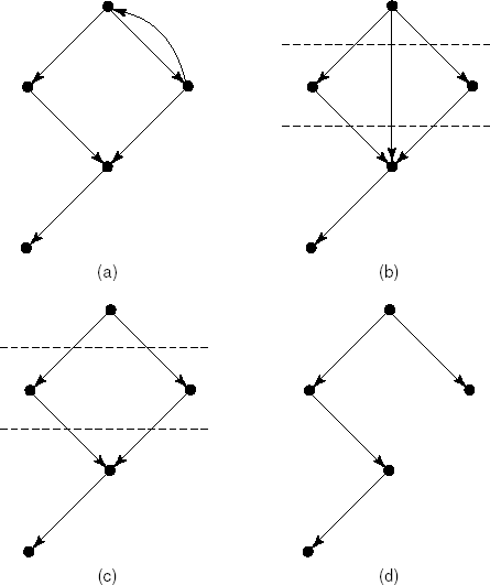
Figure 12.5. Component hierarchies: (a) directed graph, (b) directed acyclic graph, (c) layered graph, (d) tree
There are various aspects of the call graph that can be measured. Directly measurable attributes that relate to the 'shape' of the call graph include:
its size, measured in terms of the number of nodes, the number of edges, or the sum of these;
its depth, the length of the longest path from the root to some leaf node (in an acyclic directed graph);
its width, the maximum number of nodes at some level (in an acyclic directed graph).
We do not know of studies that try to quantitatively relate those measures to other complexity-related aspects such as debugging time, maintainability, etc. They may be used, though, as one of the parameters in a qualitative assessment of a design.
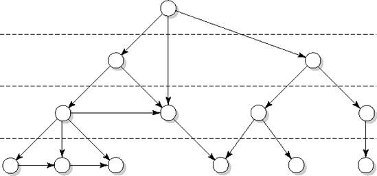
It is often stated that a good design should have a tree-like call graph. It is therefore worthwhile to consider the tree impurity of a call graph, i.e. the extent to which the graph deviates from a pure tree. Suppose we start with a connected (undirected) graph (such as the ones in Figure 12.5b-d, if we ignore the direction of the arrows). If the graph is not a tree, it has at least one cycle, i.e. a path from some node A via one or more other nodes back to A again. We may then remove one of the edges from this cycle and the result will still be a connected graph. We may continue removing edges from cycles until the result is a tree, as we did in the transition from Figure 12.5b to Figure 12.5c to Figure 12.5d. The final result is called the graph's spanning tree. The number of edges removed in this process is an indication of the graph's tree impurity.
In order to obtain a proper measure of tree impurity we proceed as follows. The complete graph Kn is the graph with n nodes and the maximum number of edges. This maximum number of edges is n(n − 1)/2. A tree with n nodes has (n − 1) edges. Given a connected graph G with n nodes and e edges, we define its tree impurity m(G) as the number of extra edges divided by the maximum number of extra edges:
This measure of tree impurity fits our intuitive notion of that concept. The value of m(G) lies between 0 and 1. It is 0 if G is a tree and 1 if it is a complete graph. If we add an edge to G, the value of m(G) increases. Moreover, the 'penalty' of extra edges is proportional to the size of the spanning tree.
It is not always easy, or even meaningful, to strive for a neat hierarchical decomposition. We will often have to settle for a compromise. It may for instance be appropriate to decompose a system into a number of clusters, each of which contains a number of components. The clusters may then be organized hierarchically, while the components within a given cluster show a more complicated interaction pattern. Also, tree-like call graphs do not allow for reuse (if a component is reused within the same system, its node in the call graph has at least two ancestors).
The call graph allows us to assess the structure of a design. In deriving the measures above, each edge in the call graph is treated alike. Yet, the complexity of the information flow that is represented by the edges is likely to vary. As noted in the earlier discussion on coupling, we would like the intercomponent connections to be 'thin'. Therefore, we would like a measure which does not merely count the edges, but which also considers the amount of information that flows through them.
The best-known attempt to measure the total level of information flow between the components of a system is due to Henri and Kafura (1981). Their measures were able to identify change-prone UNIX procedures and evaluate potential design changes. Shepperd (1990) studied the information flow measure extensively and proposed several refinements, thus obtaining a 'purer' metric. Using Shepperd's definitions, the information flow measure is based on the following notions of local and global data flow:
A local flow from component A to component B exists if
A invokes B and passes it a parameter, or
B invokes A and A returns a value.
A global flow from component A to component B exists if A updates some global data structure and B retrieves from that structure.
Using these notions of local and global data flow, Shepperd defines the 'complexity' of a component M as
where
fan-in(M) is the number of (local and global) flows whose sink is M, and
fan-out(M) is the number of (local and global) flows whose source is M.
A weak point of the information flow metric is that all flows have equal weight. Passing a simple integer as a parameter contributes equally to this measure of complexity as invoking a complex global data structure. The abstract-data-type architectural style easily results in components with a high fan-in and fan-out. If the same system is built using global data structures, its information flow metric is likely to have a smaller value. Yet, the information flow to and from the components in the abstract-data-type style generally concern simple scalar values only and are therefore considered simpler.
In a more qualitative sense, the information flow metric may indicate spots in the design that deserve our attention. If some component has a high fan-in, this may indicate that the component has little cohesion. Also, if we consider the information flow per level in a layered architecture, an excessive increase from one level to the next might indicate a missing level of abstraction.
During design, we (pre)tend to follow a top-down decomposition strategy. We may take a completely different stand and try to compose a hierarchical system structure from a flat collection of system elements. Elements that are in some sense 'closest' to one another are grouped together. We then have to define some measure for the distance between elements and a mathematical technique known as cluster analysis can be used to do the actual grouping. Elements in the same group are more like other elements within the same group and less like elements in other groups. If the measure is based on the number of data types that elements have in common, this clustering results in abstract data types or, more generally, components having high cohesion. If the measure is based on the number of data bindings between elements, the result is likely to have a low value for the information-flow metric.
The measure chosen, in a sense, determines how we define 'friendship' between elements. Close friends should be grouped in the same component while distant relatives may reside in different components. The various qualitative and quantitative design criteria that we have discussed above have different, but in essence very similar, definitions of friendship.
Though much work remains to be done, a judicious use of available design metrics is already a valuable tool in the design and quality assurance of software systems.
At the level of individual methods of an object-oriented system, we may assess quality characteristics of components by familiar metrics such as: length, cyclomatic complexity, and so on. At higher levels of abstraction, object-oriented systems consist of a collection of classes that interact by sending messages. Familiar intercomponent metrics which focus on the relationships between components do not account for the specifics of object-oriented systems. In this section, we discuss a few metrics specifically aimed at characteristics of object-oriented systems. These metrics are listed in Table 12.3.
WMC is a measure of the size of a class. The assumption is that larger classes are in general less desirable. They take more time to develop and maintain and they are likely to be less reusable. The formula is: WMC = Σni = 1 ci, where ci is the complexity of method i. For the complexity of an individual method we may choose its length, cyclomatic complexity, and so on. Most often, ci is set at 1. In that case, we simply count the number of methods. Besides being simple, this has the advantage that the metric can be applied during design, once the class interface has been decided upon. Note that each entry in the class interface counts as one method, the principle being that each method which requires additional design effort should be counted. For example, different constructors for the same operation, as is customary in C++, count as different methods.
Classes in an object-oriented design are related through a subtype — supertype hierarchy. If the class hierarchy is deep and narrow, a proper understanding of a class may require knowledge of many of its superclasses. On the other hand, a wide and shallow inheritance structure occurs when classes are more loosely coupled. The latter situation may indicate that commonality between elements is not sufficiently exploited. DIT is the distance of a class to the root of its inheritance tree. Note that the value of DIT is somewhat language-dependent. In Smalltalk, for example, every class is a subclass of Object, and this increases the value of DIT. A widely accepted heuristic is to strive for a forest of classes, i.e. a collection of inheritance trees of medium height.
NOC counts the number of immediate descendants of a class. If a class has a large number of descendants, this may indicate an improper abstraction of the parent class. A large number of descendants also suggests that the class is to be used in a variety of settings, which will make it more error-prone. The idea thus is that higher values of NOC suggest a higher complexity of the class.
CBO is the main coupling metric for object-oriented systems. Two classes are coupled if a method of one class uses a method or state variable of the other class. The CBO is a count of the number of other classes with which it is coupled. As with the traditional coupling metric, high values of CBO suggest tight bindings with other components and this is undesirable.
In the definition of CBO, all couplings are considered equal. However, if we look at the different ways in which classes may be coupled, it is reasonable to say that:
access to state variables is worse than mere parameter passing;
access to elements of a foreign class is worse than access to elements of a superclass;
passing many complex parameters is worse than passing a few simple parameters;
messages that conform to Demeter's Law[17] are better than those which do not.
If we view the methods as bubbles and the couplings as connections between bubbles, CBO simply counts the number of connections for each bubble. In reality, we consider some types of couplings worse than others: some connections are 'thicker' than others and some connections are to bubbles 'further away'. For the representation condition of measurement theory to hold, these empirical relations should be reflected in the numerical relation system.
Martin (2002) defines coupling measures at the package level:
The afferent coupling (Ca) of a package P is the number of other packages that depend upon classes within P (through inheritance or associations). It indicates the dependence of a package on its environment.
The efferent coupling (Ce) of a package P is the number of packages that classes within P depend upon. It indicates the dependence of the environment on a package.
Adding these numbers together results in a total coupling measure of a package P. The ratio I = Ce/(Ce + Ca) indicates the relative dependence of the environment to P with respect to the total number of dependencies between P and its environment. If Ce equals zero, P does not depend at all on other packages and I = 0 as well. If on the other hand Ca equals zero, P only depends on other packages and no other package depends on P. In that case, I = 1. I thus can be seen as an instability measure for P. Larger values of I denote a larger instability of the package.
RFC measures the 'immediate surroundings' of a class. Suppose a class C has a collection of methods M. Each method from M may in turn call other methods, from C or any other class. Let {Ri} be the set of methods called from method Mi. Then the response set of this class is defined as: {M} Ui {Ri}, i.e. the set of messages that may potentially be executed if a message is sent to an object of class C. RFC is defined as the number of elements in the response set. Note that we only count method calls up to one level deep. Larger values of RFC means that the immediate surroundings of a class is larger in size. There is, then, a lot of communication with other methods or classes. This makes comprehension of a class more difficult and increases test time and complexity.
The final object-oriented metric to be discussed is the lack of cohesion of a method. The traditional levels of cohesion express the degree of mutual affinity of the elements of a component. It is a measure of the glue that keeps the component together. If all methods of a class use the same state variables, these state variables serve as the glue which ties the methods together. If some methods use one subset of the state variables and other methods use another subset of the state variables, the class lacks cohesion. This may indicate a flaw in the design and it may be better to split it into two or more subclasses. LCOM is the number of disjoint sets of methods of a class. Any two methods in the same set share at least one local state variable. The preferred value for LCOM is 0.
There are obviously many more metrics that aim to address the specifics of object-oriented systems. Most of these have not been validated extensively, though. Several experiments have shown that the above set does have some merit. Overall, WMC, CBO, RFC and LCOM have been found to be the more useful quality indicators.
These metrics for example were able to predict fault-proneness of classes during design, and were found to have a strong relationship to the maintenance effort. The merits of DIT and NCO remain somewhat unclear.
Note that many of these metrics correlate with class size. One may expect that larger classes have more methods, more descendants, more couplings with other classes, etc. (El Emam et al., 2001) indeed found that class size has a confounding effect on the values of the above metrics. It thus remains questionable whether these metrics tell more than a plain LOC count.
Having discussed the properties of a good system decomposition, we now come to a question which is at least as important: how do you get a good decomposition to start with?
There exist a vast number of design methods, a sample of which are given in Table 12.4. These design methods generally consist of a set of guidelines, heuristics, and procedures on how to go about designing a system. They also offer a notation for expressing the result of the design process. Together they provide a systematic way of organizing and structuring the design process and its products.
For some methods, such as FSM or Petri nets, emphasis is on the notation, while the guidelines on how to tackle design are not very well developed. Methods such as JSD, on the other hand, offer extensive prescriptive guidelines as well. Most notations are graphical and somewhat informal, but OBJ uses a very formal mathematical language. Some methods concentrate on the design stage proper, while others, such as SSADM and JSD, are part of a wider methodology covering other life cycle phases as well. Finally, some methods offer features that make them especially useful for the design of certain types of application, such as SA/RT (for real-time systems) or Petri nets (for concurrent systems).
In the following subsections, we discuss three classical design methods:
functional decomposition, which is a rather general approach to system design, not tied to any specific method listed in Table 12.4; many different notations can be used to depict the resulting design, ranging from flowcharts or pseudocode to algebraic specifications;
data flow design, as exemplified by SA/SD;
design based on data structures, as is done in JSP and JSD.
Table 12.4. A sample of design methods
Decision tables | Matrix representation of complex decision logic at the detailed design level. |
E-R | Entity-relationship model. Family of graphical techniques for expressing data relationships; see also Chapter 10. |
Flowcharts | Simple diagram technique to show control flow at the detailed design level. Exists in many flavors; see (Tripp, 1988) for an overview. |
FSM | Finite state machine. A way to describe a system as a set of states and possible transitions between those states; the resulting diagrams are called state transition diagrams; see also Chapter 10. |
JSD | Jackson System Development; see Section 12.2.3. Successor to, and more elaborate than, JSP; has an object-oriented flavor. |
JSP | Jackson Structured Programming. Data-structure-oriented method; see Section 12.2.3. |
NoteCards | Example hypertext system. Hypertext systems make it possible to create and navigate through a complex organization of unstructured pieces of text (Conklin, 1987). |
OBJ | Algebraic specification method; highly mathematical (Goguen, 1986). |
OOD | Object-oriented design; exists in many flavors; see Section 12.3. |
Petri nets | Graphical design representation, well-suited for concurrent systems. A system is described as a set of states and possible transitions between those states. States are associated with tokens and transitions are described by firing rules. In this way, concurrent activities can be synchronized (Peterson, 1981). |
SA/SD | Structured analysis/structured design; data flow design technique; see also Section 12.2.2. |
SA/RT | Extension to structured analysis so that real-time aspects can be described (Hatley and Pirbhai, 1988). |
SSADM | Structured systems analysis and design method. A highly prescriptive method for performing the analysis and design stages; UK standard (Downs et al., 1992). |
A fourth design method, object-oriented design, is discussed in Section 12.3. Whereas the above three methods concentrate on identifying the functions of the system, object-oriented design focuses on the data on which the system is to operate. Object-oriented design is the most popular design approach today, not the least because of the omnipresence of UML as a notational device for the outcome of both requirements engineering and design.
In a functional decomposition, the intended function is decomposed into a number of subfunctions that each solve part of the problem. These subfunctions themselves may be further decomposed into yet more primitive functions, and so on. Functional decomposition is a design philosophy rather than a design method. It denotes an overall approach to problem decomposition which underlies many a design method.
With functional decomposition, we apply divide-and-conquer tactics. These tactics are analogous to, but not the same as, the technique of stepwise refinement as it is applied in 'programming in the small'. Using stepwise refinement, the refinements tend to be context-dependent. As an example, consider the following pseudo-code algorithm to insert an element into a sorted list:
procedureinsert(a, n, x);begininsert x at the end of the list; k:= n + 1;whileelementkis not at its proper placedoswap elementkand elementk- 1; k:= k-1enddo;endinsert;
The refinement of a pseudo-code instruction such as elementk is not at its proper place is done within the context of exactly the above routine, using knowledge of other parts of this routine. In the decomposition of a large system, it is precisely this type of dependency that we try to avoid. The previous section addressed this issue at great length.
During requirements engineering, the base machine has been decided upon. This base machine need not be a 'real' machine. It can be a programming language or some other set of primitives that constitutes the bottom layer of the design. During this phase too, the functions to be provided to the user have been fixed. These are the two ends of a rope. During the design phase we try to get from one end of this rope to the other. If we start from the user function end and take successively more detailed design decisions, the process is called top-down design. The reverse is called bottom-up design.
Top-down design: Starting from the main user functions at the top, we work down decomposing functions into subfunctions. Assuming we do not make any mistakes on the way down, we can be sure to construct the specified system. With top-down design, each step is characterized by the design decisions it embodies. To be able to apply a pure top-down technique, the system has to be fully described. This is hardly ever the case. Working top-down also means that the earliest decisions are the most important ones. Undoing those decisions can be very costly.
Bottom-up design: Using bottom-up design, we start from a set of available base functions. From there we proceed towards the requirements specification through abstraction. This technique is potentially more flexible, especially since the lower layers of the design could be independent of the application and thus have wider applicability. This is especially important if the requirements have not been formulated very precisely yet or if a family of systems has to be developed. A real danger of the bottom-up technique is that we may miss the target.
In their pure form, neither the top-down nor the bottom-up technique is likely to be used all that often. Both techniques are feasible only if the design process is a pure and rational one. And this is an idealization of reality. There are many reasons why the design process cannot be rational. Some of these have to do with the intangibles of design processes per se, some originate from accidents that befall many a software project. Parnas and Clements (1986) list the following reasons, amongst others:
Mostly, users do not know exactly what they want and they are not able to tell all they know.
Even if the requirements are fully known, a lot of additional information is needed. This information is discovered only when the project is under way.
Almost all projects are subject to change. Changes influence earlier decisions.
People make errors.
During design, people use the knowledge they already have, experiences from earlier projects, and so on.
In many projects, we do not start from scratch — we build from existing software.
Design exhibits a 'yo-yo' character: something is devised, tried, rejected again, new ideas crop up, etc. Designers frequently go about in rather opportunistic ways. They frequently switch from high-level, application domain issues to coding and detailed design matters, and use a variety of means to gather insight into the problem to be solved. At most, we may present the result of the design process as if it came about through a rational process.
A general problem with any form of functional decomposition is that it is often not immediately clear along which dimension the system is decomposed. If we decompose along the time axis, the result is often a main program that controls the order in which a number of subordinate components is called. In Yourdon's classification, the resulting cohesion type is temporal. If we decompose with respect to the grouping of data, we obtain the type of data cohesion exhibited in abstract data types. Both these functional decompositions can be viewed as an instance of some architectural style. Rather than worrying about which dimension to focus on during functional decomposition, you had better opt for a particular architectural style and let that style guide the decomposition.
At some intermediate level, the set of interrelated components comprises the software architecture as discussed in Chapter 11. This software architecture is a product which serves various purposes: it can be used to discuss the design with different stakeholders; it can be used to evaluate the quality of the design; it can be the basis for the work-breakdown structure; it can be used to guide the testing process, etc. If a software architecture is required, it necessitates a design approach in which, at quite an early stage, every component and connection is present. A bottom-up or top-down approach does not meet this requirement, since in both these approaches only part of the solution is available at intermediate points in time.
Parnas (1978) offers the following useful guidelines for a sound functional decomposition:
Try to identify subsystems. Start with a minimal subset and define minimal extensions to this subset.
The idea behind this guideline is that it is extremely difficult, if not impossible, to get a complete picture of the system during requirements engineering. People ask too much or they ask the wrong things. Starting from a minimal subsystem, we may add functionality incrementally, using the experience gained with the actual use of the system. The idea is very similar to that of agile approaches, discussed in Chapter 3.
Apply the information-hiding principle.
Try to define extensions to the base machine step by step.
This holds for both the minimal machine and its extensions. Such incremental extensions lead to the concept of a virtual machine. Each layer in the system hierarchy can be viewed as a machine. The primitive operations of this machine are implemented by the lower layers of the hierarchy. This machine view of the component hierarchy nicely maps onto a layered architectural style. It also adds a further dimension to the system structuring guidelines offered in Section 12.1.5.
Apply the uses relation and try to place the dependencies thus obtained in a hierarchical structure.
Obviously, the above guidelines are strongly interrelated. It has been said before that a strictly hierarchical tree structure of system components is often not feasible. A compromise that often is feasible is a layered system structure as depicted in Figure 12.6.
The arrows between the various nodes in the graph indicate the uses relation. Various levels can be distinguished in the structure depicted. Components at a given level only use components from the same, or lower, levels. The layers distinguished in Figure 12.6 are not the same as those induced by the acyclicity of the graph (as discussed in Section 12.1.5) but are rather the result of viewing a distinct set of components as an abstract, virtual machine. Deciding how to group components into layers in this way involves considering the semantics of those components. Lower levels in this hierarchy bring us closer to the 'real' machine on which the system is going to be executed. Higher levels are more application-oriented. The choice of the number of levels in such an architecture is a (problem-dependent) design decision.
This work of Parnas heralds some of the notions that were later recognized as important guiding principles in the field of software architecture. The idea of a minimal subset to which extensions are defined is very similar to the notion of a product-line architecture: a basic architecture from which a family of similar systems can be derived. The layered approach is one of the basic architectural styles discussed in Section 11.4.
The data flow design method originated in the early 1970s with Yourdon and Constantine. In its simplest form, data flow design is but a functional decomposition with respect to the flow of data. A component is a black box which transforms some input stream into some output stream. In data flow design, heavy use is made of graphical representations known as data flow diagrams (DFDs) and structure charts. Data flow diagrams were introduced as a modeling notation in Section 10.1.3.
Data flow design is usually seen as a two-step process. First, a logical design is derived in the form of a set of data flow diagrams. This step is referred to as structured analysis (SA). Next, the logical design is transformed into a program structure represented as a set of structure charts. The latter step is called structured design (SD). The combination is referred to as SA/SD.
Structured analysis can be viewed as a proper requirements engineering method insofar as it addresses the modeling of some universe of discourse (UoD). It should be noted that, as data flow diagrams are refined, the analyst performs an implicit (top-down) functional decomposition of the system as well. At the same time, the diagram refinements result in corresponding data refinements. The analysis process thus has design aspects as well.
Structured design, being a strategy to map the information flow contained in data flow diagrams into a program structure, is a genuine component of the (detailed) design phase.
The main result of structured analysis is a series of data flow diagrams. Four types of data entity are distinguished in these diagrams:
External entities are the source or destination of a transaction. These entities are located outside the domain considered in the data flow diagram. External entities are indicated as squares.
Processes transform data. Processes are denoted by circles.
Data flows between processes, external entities, and data stores. A data flow is indicated by an arrow. Data flows are paths along which data structures travel.
Data stores lie between two processes. This is indicated by the name of the data store between two parallel lines. Data stores are places where data structures are stored until needed.
We illustrate the various process steps of SA/SD by analyzing and designing a simple library automation system. The system allows library clients to borrow and return books. It also reports to library management about how the library is used by its clients (for example, the average number of books on loan and authors much in demand).
At the highest level, we draw a context diagram, a data flow diagram with one process, denoting 'the system'. Its main purpose is to depict the interaction of the system with the environment (the collection of external entities). For our simple library system, this is done in Figure 12.7. This diagram has yet to be supplemented by a description of the structure of both the input and output to the central process.
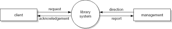
Next, this top-level diagram is further decomposed. For our example, this could lead to the data flow diagram of Figure 12.8 (which is the same as Figure 10.3). In this diagram, we have expanded the central process node of the context diagram. A client request is first analyzed in a process labeled 'preliminary processing'. As a result, one of 'borrow title' or 'return title' is activated. Both these processes update a data store labeled 'catalog administration'. Client requests are logged in a data store 'log file'. This data store is used to produce management reports.

For more complicated applications, various diagrams could be drawn, one for each subsystem identified. These subsystems in turn are further decomposed into diagrams at yet lower levels. We thus get a hierarchy of diagrams. As an example, a possible refinement of the 'preliminary processing' node is given in Figure 12.9. In lower-level diagrams, the external entities are usually omitted.
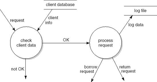
The top-down decomposition stops when a process becomes sufficiently straightforward and does not warrant further expansion. These primitive processes are described in minispecs. A minispec serves to communicate the algorithm of the process to relevant parties. It may use notations such as structured natural language, pseudocode, or decision tables. Example screen layouts can be added to illustrate how the input and output will look. An example minispec for 'process request' is given in Figure 12.10.
The contents of the data flows in a DFD are recorded in a data dictionary. Though this name suggests something grand, it is nothing more than a precise description of the structure of the data. This is often done in the form of regular expressions, such as the example in Figure 12.11. Nowadays, the static aspects of the data tend to be modeled in ER diagrams; see Chapter 10.
The result of structured analysis is a logical model of the system. It consists of a set of DFDs, augmented by descriptions of its constituents in the form of minispecs, formats of data stores, and so on. In the subsequent structured design step, the data flow diagrams are transformed into a collection of components (subprograms) that call one another and pass data. The result of the structured design step is expressed in a hierarchical set of structure charts. There are no strict rules for this step. Textbooks on the data flow technique give guidelines, and sometimes even well-defined strategies, for how to get from a set of data flow diagrams to a hierarchical model for the implementation. These guidelines are strongly inspired by the various notions discussed in Section 12.1, most notably cohesion and coupling.
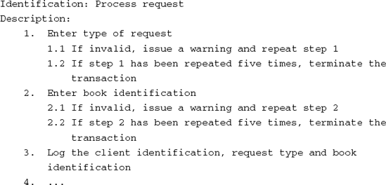
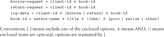
The major heuristic involves the choice of the top-level structure chart. Many data-processing systems are essentially transform-centered: input is read and possibly edited, a major transformation is done, and the result is output. One way to decide upon the central transformation is to trace the input through the data flow diagram until it can no longer be considered input. The same is done, in the other direction, for the output. The bubble in between is as the central transform. If we view the bubbles in a DFD as beads, and the data flows as threads, we obtain the corresponding structure chart by picking the bead that corresponds to the central transformation and shaking the DFD.[18] The processes in the data flow diagram become the components of the corresponding structure chart and the data flows become component invocations. Note that the arrows in a structure chart denote component invocations, whereas the arrows in a data flow diagram denote flows of data. These arrows often point in opposite directions; a flow of data from A to B is often realized through an invocation of A by B. Sometimes it is difficult to select one central transformation. In that case, a dummy root element is added and the resulting input-process-output scheme is of the form depicted in Figure 12.12.
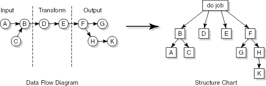
Because of the transformation orientation of the structure chart, the relations between components in the graph have a producer-consumer character. One component produces a stream of data which is then consumed by another component. The control flow is one whereby components invoke subordinate components so as to realize the required transformation. There is a potentially complex stream of information between components, corresponding to the data flow that is passed between producer and consumer.
The major contribution of structured design is found in the guidelines that aim to reduce the complexity of the interaction between components. These guidelines concern the cohesion and coupling criteria discussed in Section 12.1.
The best-known technique for design based on data structures originated with Jackson (1975). The technique is known as Jackson Structured Programming (JSP). Essentials of JSP have been carried over to Jackson System Development (JSD). JSP is a technique for programming-in-the-small and JSD is a technique for programming-in-the-large. We discuss both techniques in turn.
The basic idea of JSP is that a good program reflects the structure of both the input and the output in all its facets. Given a correct model of the data structures, we may straightforwardly derive the corresponding program from the model. It is often postulated that the structure of the data is much less volatile than the transformations applied to the data. As a consequence, designs that take the data as their starting point should be 'better' too. This same argument is also used in the context of object-oriented analysis and design.
JSP distinguishes elementary and compound components. Elementary components are not further decomposed. There are three types of compound component: sequence, iteration and selection. Compound components are represented by diagrams (also called Jackson diagrams or structure diagrams) or some sort of pseudocode (called structure text or schematic logic). The base form of both representations are given in Figure 12.13. In the structure text, 'seq' denotes sequencing, 'itr' denotes iteration, 'sel' denotes selection, and 'alt' denotes alternatives.
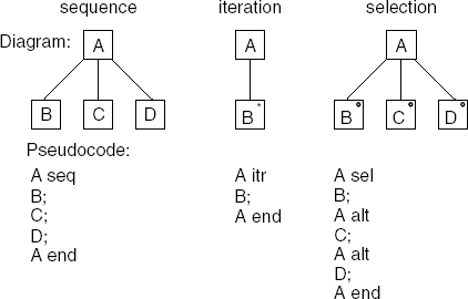
Most modern programming languages have structures (loops, if statements and sequential composition) for each of these diagrammatic notations or, for that matter, the corresponding pseudocode for the structure of data. The essence of Jackson's technique is that the structure diagrams of the input and output can be merged, thus yielding the global structure of the program.
To illustrate this line of thought, consider a fragment from a library system. The system keeps track of which books from which authors are being borrowed (and returned). From this log, we want to produce a report that lists how often each title is borrowed. Using Jackson's notation, the input for this function could be as specified in Figure 12.14.[19] A possible structure for the output is given in Figure 12.15.
The program diagram to transform the log into a report is obtained by merging the two diagrams; see Figure 12.16. The structure of the resulting program can be derived straightforwardly from this diagram (see Figure 12.17).
This merging of diagrams does not work for the lower levels of our problem, 'process mutation' and its subordinate nodes. The cause is something called a structure clash: the input and output data structures do not really match. The reason is that the input consists of a sequence of mutations. In the output, all mutations for a given book are taken together. So, the mutations have to be sorted first. We have to restructure the system, for instance as depicted in Figure 12.18.
A clear disadvantage of the structure thus obtained is that there is now an intermediate file. Closer inspection shows that we do not really need this file. This is immediately clear if we depict the structure as in Figure 12.19.
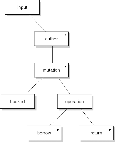
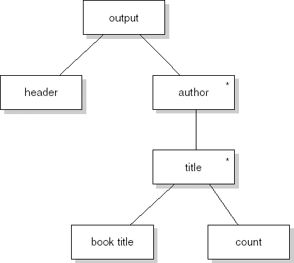
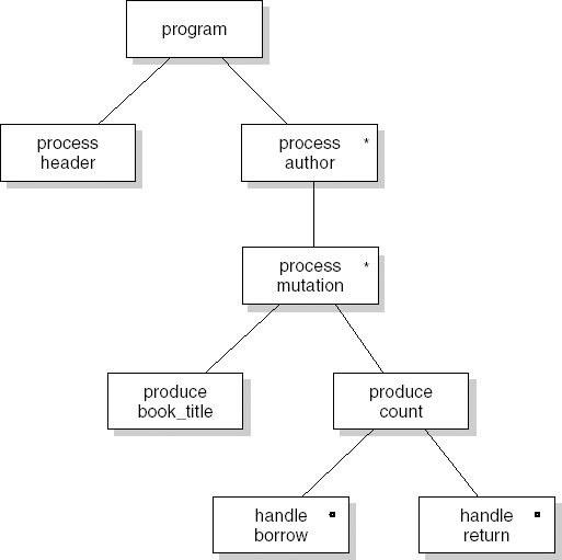
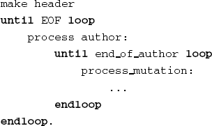
Here, we may invert component A1 and code it such that it serves as a replacement of component B2. Alternatively (and in this case more likely), we may invert B1 and substitute the result for component A2. In either case, the first-in-first-out (FIFO) type of intermediate file between the two components is removed by making one of the components a subordinate of the other.
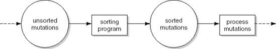
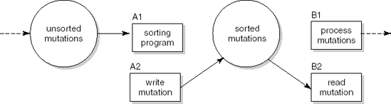
This example shows the fundamental issues involved in the use of JSP:
modeling input and output using structure diagrams,
merging the diagrams to create the program structure, meanwhile
resolving possible structure clashes, and finally
optimizing the result through program inversion.
If we choose a linear notation for the structure diagrams, the result falls into the class of 'regular expressions'. Thus, the expressive power of these diagrams is that of a finite automaton. Some of the structure clashes crop up if the problem cannot be solved by a finite automaton.
Both in the functional decomposition and in the data flow design methods, the problem structure is mapped onto a functional structure. This functional structure is next mapped onto a program structure. In contrast, JSP maps the problem structure onto a data structure and the program structure is derived from this data structure. JSP is not much concerned with the question of how the mapping from problem structure to data structure is obtained.
Jackson System Development (JSD) tries to fill this gap. JSD distinguishes three stages in the software development process:
A modeling stage in which a description is made of the real-world problem through the identification of entities and actions;
A network stage in which the system is modeled as a network of communicating concurrent processes;
An implementation stage in which the network of processes is transformed into a sequential design.
The first step in JSD is to model the part of reality we are interested in, the UoD. JSD models the UoD as a set of entities, objects in the real world that participate in a time-ordered sequence of actions. For each entity, a process is created which models the life cycle of that entity. Actions are events that happen to an entity. For instance, in a library the life cycle of an entity Book could be as depicted in Figure 12.20. The life cycle of a book starts when it is acquired. After that it may be borrowed and returned any number of times. The life cycle ends when the book is either archived or disposed of. The life cycle is depicted using process structure diagrams (PSDs). PSDs are hierarchical diagrams that resemble the structure diagrams of JSP, with its primitives to denote concatenation (ordering in time), repetition, and selection. PSDs have a pseudocode equivalent called structure text which looks like the schematic logic of JSP.
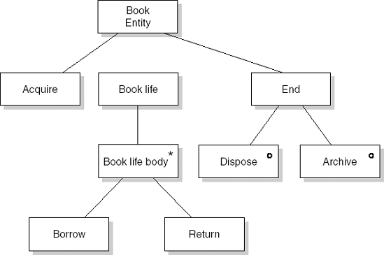
Process structure diagrams are finite state diagrams. In traditional finite state diagrams, the bubbles (nodes) represent possible states of the entity being modeled while the arrows denote possible transitions between states. The opposite is true for PSDs. In a PSD, nodes denote state transitions and arrows denote states.
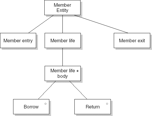
Following this line of thought, an entity Member can be described as in Figure 12.21: members enter the library system, after which they may borrow and return books until they cease to be a member.
The modeling stage is concerned with identifying entities and the events (actions) that happen to them. These actions collectively constitute the life cycle of an entity. As with other design methods, there is no simple recipe to determine the set of entities and actions. The approach generally taken has a linguistic stance. From notes, documentation, interviews and the like, we may draw up a preliminary list of actions and entities. One heuristic is to look for real-world objects with which the system is to interact. Since a library is all about books, an entity Book immediately suggests itself. From statements such as 'members borrow books', we may infer that an event Borrow occurs in the life cycle of both books and members. Once such a preliminary list is made up, further reflection should lead to a precisely demarcated life cycle of the entities identified.
Entities are made up of actions. These actions are atomic, i.e. they cannot be further decomposed into subactions. Actions respond to events in the real world. The action Acquire that is part of the life cycle of the entity Book is triggered when a real-world event, the actual acquisition of a book, takes place. In the process structure diagram, actions show up as leaf nodes.
Events are communicated to the system through data messages, called attributes. In a procedural sense, these attributes constitute the parameters of the action. For the action Acquire, we may have such attributes as ISBN, date-of-acquisition, title and authors.
Entities have attributes as well: local variables that keep information from the past and collectively determine its state. The entity Book for example may retain some or all of the information that was provided upon acquisition (for example, ISBN, title). Entities also have two special attributes. First, the identifier attribute uniquely identifies the entity. Second, each entity has an attribute that indicates its status. This attribute can be viewed as a pointer to some leaf node of the process structure diagram.
Each entity can be viewed as a separate, long-running, process. In the library example, each book and each member has its own life cycle. The processes though are not completely independent. During the network stage, the system is modeled as a network of interconnected processes. This network is depicted in a system specification diagram (SSD). JSD has two basic mechanisms for interprocess communication:
An entity may inspect the state vector of another entity. This state vector describes the local state of an entity at some point in time.
An entity may asynchronously pass information to another entity through a datastream.
Recall that the actions Borrow and Return occur in the life cycle of both Book and Member (see Figures 12.20 and 12.21). Such common actions create a link between these entities. As a consequence, the life cycles of these entities are synchronized with respect to these events.
If a member wants to borrow a book, certain information about that book is required. A Member entity may obtain that information by inspecting the state vector of the appropriate Book entity. This type of communication is indicated by the diamond in Figure 12.22. In an implementation, state vector communication is usually handled through database access.
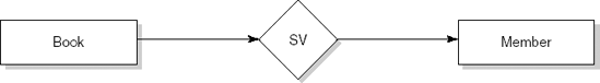
If our system is to log information on books being borrowed, we may model this by means of a datastream from an entity Book to an entity Log. A datastream is handled on a FIFO basis; it behaves like the UNIX filter. The notation for the datastream type of communication is given in Figure 12.23.
The final stage of JSD is the implementation stage, in which the concurrent model that is the result of the network stage is transformed into an executable system. One of the key concepts for this stage is program inversion: the communication between processes is replaced by a procedure call, so that one process becomes a subordinate of another process. This is very similar to the notion of program inversion as present in JSP.
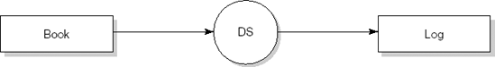
The key concepts that play a role in the object-oriented approach to analysis and design have been mentioned already in Chapter 10: objects, their attributes and services, and the relationships between objects. It follows quite naturally from the above that the object-oriented approach to systems analysis and design involves three major steps:
Identify the objects;
Determine their attributes and services;
Determine the relationships between objects.
Obviously, these steps are highly interrelated and some form of iteration will be needed before the final design is obtained. The resulting picture of the system as a collection of objects and their interrelationships describes the static structure (decomposition) of the system. This static model is graphically depicted in some variant of the class diagram as described in Section 10.3.1.
An object instance is created, updated zero or more times, and finally destroyed. Finite state diagrams depicting the possible states of an object and the transitions between those states are a good help in modeling this life cycle. Object-oriented methods generally use some variant of the state machine diagram of UML to show this dynamic model of the behavior of system components; see Section 10.3.2.
Components of the system communicate by sending messages. These messages are part of a task that the system has to perform. We may find out which messages are needed, and in which order they have to be exchanged, by considering typical usage scenarios. Scenario analysis is a requirements elicitation technique. In object-oriented circles, this technique is known as use-case analysis. The resulting model of the communication between system components is depicted in a sequence or communication diagram; see Sections 10.3.3 and 10.3.4. These views are also part of the dynamic model.
The guidelines for finding objects and their attributes and services are mostly linguistic in nature, much like the ones mentioned in our discussion of JSD in Section 12.2.3. Indeed, the modeling stage of JSD is object-oriented too. The guidelines presented below are loosely based on (Coad and Yourdon, 1991) and (Rumbaugh et al., 1991). Their general flavor is similar to that found in other object-oriented approaches. The global process models of some well-known object-oriented methods are discussed in Sections 12.3.1 and 12.3.2.
The problem statement for a library automation system given in Figure 12.24 will serve as an example to illustrate the major steps in object-oriented analysis and design. We will elaborate part of this problem in the text, and leave a number of detailed issues as exercises.
A major guiding principle for identifying objects is to look for important concepts from the application domain. Objects to be found in a library include Books, FileCabinets, Customers, etc. In an office environment, we may have Folders, Letters, Clerks, etc. These domain-specific entities are our prime candidates for objects. They may be real-world objects, such as a book; roles played, such as the customer of a library; organizational units, such as a department; locations, such as an office; or devices, such as a printer. Potential objects can also be found by considering existing classification or assembly (whole-part) structures. From interviews, documentation, and so on, a first inventory of objects can be made.
From the first paragraph of the problem description in Figure 12.24, the following list of candidate objects can be deduced, simply by listing all the nouns:
software
library
system
station
customer
transaction
book
library employee
identification card
client
bar code reader
book's code
Some objects on this candidate list should be eliminated:
Software, for example, is an implementation construct which should not be included in the model at this point in time. A similar fate should befall terms such asalgorithmandlinked list. At the detailed design stage, there may be reasons to introduce (or reintroduce) them as solution-oriented objects.Vague terms should be replaced by more concrete terms or eliminated.
Systemis a vague term in our candidate list. The stations and PCs will be connected to the same host computer, so we might as well use the notioncomputerinstead ofsystem.Customerandclientare synonymous terms in the problem statement. Only one of them is therefore retained. We must be careful in how we modelclientandlibrary employee. One physical person may assume both roles. Whether it is useful to model these as distinct objects or as different roles of one object is difficult to decide at this point. We will treat them as separate objects for now, but keep in mind that this may change when the model is refined.The term
transactionrefers to an operation applied to objects, rather than an object in itself. It involves a sequence of actions such as handing an identification card and a book copy to the employee, inserting the identification card into the station, reading the book's bar code, and so on. Only if transactions themselves have features which are important to the system should they be modeled as objects. For instance, if the system has to produce profile information about client preferences, it may be useful to have an objecttransaction.The term
bookis a bit tricky in this context. A book in a library system may denote both a physical copy and an abstract key denoting a particular {author, title} combination. The former meaning is intended when we speak about the borrowing of a book, while the latter is intended where it concerns entries in the library catalog. Inexperienced designers may equate these interpretations and end up with the wrong system. We are interested (in this part of the system) in modeling book copies.The
book's codedescribes an individual object rather than a class of objects. It should be restated as an attribute of the objectbook copy.
Figure 12.25 lists the relationships between objects that can be inferred from the problem statement in Figure 12.24. These relationships are directly copied from the problem statement or are part of the tacit knowledge we have of the domain.
The resulting objects and relationships are included in the initial class diagram of Figure 12.26. We have only included the names of the relationships in this diagram. Further adornments, such as cardinality constraints and specialization-generalization information, may be included when the model is refined.
We next identify the attributes of objects. Attributes describe an instance of an object. Collectively, the attributes constitute the state of the object. Attributes are identified by considering the characteristics that distinguish individual instances, yet are common properties of the instances of an object type. We thus look for atomic attributes rather than composite ones. For our library customer, we would for example obtain attributes Name and Address rather than a composite attribute NameAnd-Address. At this stage, we also try to prevent redundancies in the set of attributes. So rather than having attributes BooksOnLoan and NumberOfBooksOnLoan, we settle for the former only, since the latter can be computed from that attribute.
The major services provided by an object are those that relate to its life cycle. For example, a copy of a book is acquired, is borrowed and returned zero or more times, and finally goes out of circulation. A person becomes a member of the library member-of library and may borrow and return books, reserve titles, change address, pay fines, and so on, until he finally ceases to be a member.
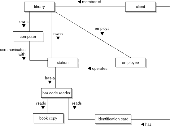
These services concern the state of an object: they read and write the object's attributes. Services that provide information about the state of an object may or may not involve some type of computation. Note that it is always possible to optimize the actual implementation by keeping redundant information in the state as it is maintained by the object. For example, we may decide to include the number of books on loan in the state as implemented, rather than computing it when required. This need not concern us at this stage though. Whether services are actually implemented by computational means or by a simple lookup procedure is invisible to the object that requests the information.
Further insight into which services are required can be obtained by investigating usage scenarios. We may prepare typical dialogs between components of the system in both normal and exceptional situations. For example, we may consider the situation in which a client successfully borrows a book, one in which the client's identification card is no longer valid, one in which he still has to pay an outstanding fine, and so on. A sequence diagram for the normal situation of borrowing a book is shown in Figure 12.27. A number of events take place when this interaction takes place. These events will be handled by operations of the objects involved.
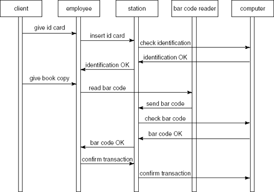
Services are but one way through which objects may be related. The relations which give systems a truly object-oriented flavor are those which result from whole-part and specialization-generalization classifications.
Part of the classification of objects may result from the pre-existing real-world classifications that the system is to deal with. Further classification of objects into an object hierarchy involves a search for relations between objects. To start with, we may consider an object as a generalization of other possible objects. For instance, the object Book may be viewed as a generalization of the objects Novel, Poetry and ReferenceBook. Whether these specializations are meaningful depends on the problem at hand. If the system does not need to distinguish between novels and poetry, we should not define separate objects for them. The distinction between novels and poetry on the one hand and reference books on the other is sensible, though, if novels and poetry can be borrowed, but reference books cannot.
In a similar way, we may consider similarities between objects, thus viewing them as specializations of a more general object. If our library system calls for objects Book and Journal that have a number of attributes in common, we may introduce a new object Publication as a generalization of these objects. The common attributes are lifted to the object Publication; Book and Journal then inherit these attributes. Note that generalizations should still reflect meaningful real-world entities. There is no point in introducing a generalization of Book and FileCabinet simply because they have a common attribute of Location.
The object Publication is an abstract object. It is an object for which there are no instances. The library only contains instances of objects that are a specialization of Publication, such as Book and Journal. Its function in the object hierarchy is to relate these other objects and to provide an interface description to its users. The attributes and services defined at the level of Publication together constitute the common interface for all its descendants.
The specialization-generalization hierarchy also makes it possible to lift services to higher levels of the hierarchy. Doing so often gives rise to so-called virtual functions. Virtual functions are services of an object for which a (default) implementation is provided which can be redefined by specializations of that object. The notion of virtual functions greatly enhances reusability, since a variant of some object can now be obtained by constructing a specialization of that object in which some services are redefined.
Decisions as to which objects and attributes to include in a design, and how to relate them in the object hierarchy, are highly intertwined. For instance, if an object has only one attribute, it is generally better to include it as an attribute in other objects. Also, the instances of an object should have common attributes. If some attributes are only meaningful for a subset of all instances, then we really have a classification structure. If some books can be borrowed, but others cannot, this is an indication of a classification structure where the object Book has specializations such as Novel and ReferenceBook.
Note also that, over time, the set of attributes of and services provided by an object tends to evolve, while the object hierarchy remains relatively stable. If our library decides to offer an extra service to its customers, say borrowing records, we may simply adapt the set of attributes and extend the set of services for the object Customer.
Object-oriented design can be classified as a middle-out design method. The set of objects identified during the first modeling stages constitutes the middle level of the system. In order to implement these domain-specific entities, lower-level objects are used. These lower-level objects can often be taken from a class library. For the various object-oriented programming languages, quite extensive class libraries already exist. The higher levels of the design constitute the application-dependent interaction of the domain-specific entities.
In the following subsections, we discuss three design methods that typify the evolution of object-oriented analysis and design:
the Booch method, an early object-oriented analysis and design method, with an emphasis on employing a new and rich set of notations;
Fusion, developed at HP, with a much larger emphasis on the various process steps of the method;
the Rational Unified Process (RUP), a full life cycle model associated with UML.
The global process model of the method described in (Booch, 1994) is shown in Figure 12.28. It consists of four steps, to be carried out in roughly the order shown. The process is iterative, so each of the steps may have to be done more than once. The first cycles are analysis-oriented, while later ones are design-oriented. The blurring of activities in this process model is intentional. Analysis and design activities are assumed to be under opportunistic control. It is therefore not deemed realistic to prescribe a purely rational order for the activities to be carried out.
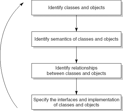
Figure 12.28. The process model of Booch (Source: G. Booch, Object-Oriented Analysis and Design, ©1994, Benjamin Cummings Publishing Company. Reproduced by permission of Addison Wesley Longman.)
The first step is aimed at identifying classes and objects. The purpose of this step is to establish the boundaries of the problem and to obtain a first decomposition. During analysis, the emphasis is on finding meaningful abstractions from the application domain. During design, objects from the solution domain may be added. The major outcome of this step is a data dictionary containing a precise description of the abstractions identified.
The second step is concerned with determining the behavior and attributes of each abstraction, and the distribution of responsibilities over components of the system. Attributes and desired behavior are identified by analyzing typical usage scenarios. As this process proceeds, responsibilities may be reallocated to get a more balanced design, or be able to reuse (scavenge) existing designs. The outcome of this step is a reasonably complete set of responsibilities and operations for each abstraction. The results are documented in the data dictionary and, at a later stage, in interface specifications for each abstraction. The semantics of usage scenarios are captured in sequence and communication diagrams (termed interaction diagrams and object diagrams, respectively, in (Booch, 1994)).
The third step is concerned with finding relationships between objects. During analysis, the emphasis is on finding relationships between abstractions. During design, tactical decisions about inheritance, instantiation, and so on are made. The results are shown in class diagrams, communication diagrams, and 'module diagrams', which show the modular structure of a system.
Finally, the abstractions are refined to a detailed level. A decision is made about the representation of each abstraction, algorithms are selected, and solution-oriented classes are added where needed.
The most notable characteristics of Booch's method are:
A rich set of notations: it uses six types of diagram, each with a fairly elaborate vocabulary; as a result, many aspects of a system can be modeled
A poor process model: it is difficult to decide when to iterate, and what to do in a specific iteration.
The Fusion method for object-oriented analysis and design has two major phases: analysis and design. Its global process model is shown in Figure 12.29.
The analysis phase is aimed at determining the system's objects and their interactions. The static structure is shown in a class diagram (called an object model in Fusion) and documented in a data dictionary. The dynamics are shown in the interface model. The interface model consists of a life cycle model for each object, denoted by a regular expression (i.e., a flat representation of a state machine diagram) and a specification of the semantics of each operation in a pre- and postcondition style. The analysis process is assumed to be an iterative process. This iteration stops when the models are complete and consistent.
Fusion's design phase results in four models, which are essentially derived in the order indicated in Figure 12.29. Object interaction graphs resemble communication graphs. They describe how objects interact at run time: what objects are involved in a computation and how they are combined to realize a given specification. Visibility graphs describe how the communications between objects are realized. For each object, it is determined which other objects must be referenced and how. Different kinds of references are distinguished, taking into account aspects such as the lifetime of the reference and whether references can be shared. Next, the object model, interaction graphs, and visibility graphs are used to derive a description of each class. The operations and the initial set of attributes for each object are established at this stage. Finally, the inheritance relations are decided upon and depicted in the inheritance graph, which is a class diagram. The class descriptions are then updated to reflect this inheritance structure.
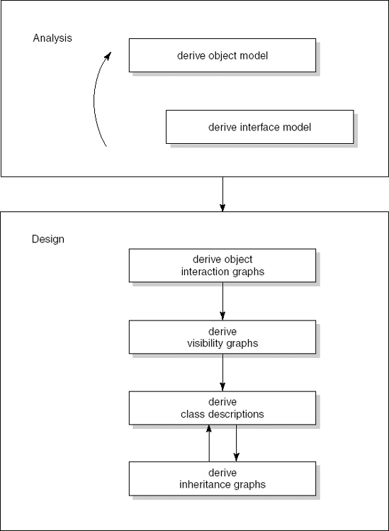
The most notable characteristics of Fusion are:
A large amount of attention is paid to the design phase. Fusion defines four models for the design phase and gives detailed guidelines for the kind of things that have to be incorporated in these models.
The version of the method as published in (Coleman et al., 1994) hinges on the availability of a good requirements document. Extensions to this version include the absorption of use cases to drive the analysis process.
As a method, Fusion is very prescriptive. The contrast with the opportunistic approach of Booch is striking. Fusion's prescriptiveness might be considered both a strength and a weakness.
The Rational Unified Process (RUP) is a full process model; see also Section 3.3. RUP has a number of workflows, such as a requirements workflow, analysis and design workflow, and test workflow, and four phases: inception, elaboration, construction, and transition. Workflows describe the activities to be carried out, while the phases indicate the organization along the time axis. Most workflows extend over most phases.
Here, we discuss the analysis and design workflow, in which the requirements are transformed into a design. RUP is an iterative process, so this transformation is carried out in a number of iterations as well. The first iterations take place in the elaboration phase of RUP. In that phase, the architecture of the system is determined. The RUP way of doing architectural design reasonably fits the global workflow model discussed in Section 11.2. In subsequent iterations, concerning the lower-level design, the main activities are analyze behavior and design components.
The purpose of the analyze behavior step is to transform the use cases into a set of design elements that together serve as a model of the problem domain. It is about what the system is to deliver. It produces a black-box model of the solution. The purpose of the design elements step is to refine the definitions of the design elements into classes, relationships, interfaces, and so on. In this activity, the black-box, what model is turned into a white-box, how model.
During both activities, the design is reviewed and the results are fed back into the next iteration.
Notable characteristics of RUP are:
It is a very complete, iterative model that goes much further than mere analysis and design.
It makes heavy use of UML to represent artifacts and views.
Use cases play a central role. They provide thread information from one workflow to another. For example, the analysis and design workflow produces use-case realizations, which describe how use cases are actually realized by a collection of interacting objects and classes.
It is not easy to compare the many design methods that exist. They all have their pros and cons. None of them gives us a straightforward recipe as to how to proceed from a list of requirements to a successfully implemented system. We always need some sort of magic in order to get a specific decomposition. The expertise and quality of the people involved have a major impact on the end result of the design process.
Problem solving is based on experience. It is estimated that an expert has over 50 000 chunks of domain-specific knowledge at his disposal. When solving a problem, we try to map the problem at hand onto the knowledge available. The greater this knowledge is, and the more accessible it is, the more successful this process will be.
The prescriptiveness of the design methods differs considerably. The variants of functional decomposition and the object-oriented design methods rely heavily on the heuristic knowledge of the designers. Jackson's techniques seem to suffer less from this need. Especially if structure clashes do not occur, JSP provides a well-defined framework for tackling design. The prescriptive nature of JSP possibly explains to some extent its success in the past, especially in the realm of administrative data processing. JSD offers similar advantages. Its strict view of describing data structures as a list of events may lead to problems, however, if the data structures do not fit this model. JSP has a static view of the data. More importantly, it does not tell us how to organize the data. As such, this technique seems most suited to problems where the structure of the data has been fixed beforehand. JSD and object-oriented methods offer better support as regards the structuring of data. Though these methods give useful heuristics for the identification of objects, obtaining a well-balanced set of objects is still very much dependent on the skills of the designer.
The data flow technique has a more dynamic view of the datastreams that are the base of the system to be constructed. We may often view the bubbles from a data flow diagram as clerks that perform certain transformations on incoming data to produce data for other clerks. The technique seems well-suited for circumstances where an existing manual system is to be replaced by a computerized one. A real danger, though, is that the existing system is just copied, while additional requirements are overlooked.
If we take into account that a substantial part of the cost of software is spent in maintaining that software, it is clear that such factors as flexibility, comprehensibility, and modularity should play a crucial role when selecting a specific design technique. The ideas and guidelines of Parnas are particularly relevant in this respect. The object-oriented philosophy incorporates these ideas and is well-matched to current programming languages, which allow for a smoother transition between the different development phases.
Quite a few attempts have been made to classify design methods along various dimensions, such as the products they deliver, the kind of representations used, or their level of formality. A simple but useful framework is proposed in (Blum, 1994). It has two dimensions: an orientation dimension and a model dimension.
In the orientation dimension, a distinction is made between problem-oriented techniques and product-oriented techniques. Problem-oriented techniques concentrate on producing a better understanding of the problem and its solution. Problem-oriented techniques are human-oriented. Their aim is to describe, communicate, and document decisions. Problem-oriented techniques usually have one foot in the requirements engineering domain. Conversely, product-oriented techniques focus on a correct transformation from a specification to an implementation. The second dimension relates to the products, i.e. models, that are the result of the design process. In this dimension, a distinction is made between conceptual models and formal models. Conceptual models are descriptive. They describe an external reality, the universe of discourse. Their appropriateness is established through validation. Formal models on the other hand are prescriptive. They prescribe the behavior of the system to be developed. Formal models can be verified.
Using this framework, we may classify a number of techniques discussed in this book as in Table 12.5. The four quadrants of this matrix have the following characteristics:
Understand the problem These techniques are concerned with understanding the problem and expressing a solution in a form that can be discussed with domain specialists (i.e. the users).
Transform to implementation Techniques in this category help to transform a collection of UoD-related concepts into an implementation structure.
Represent properties These techniques facilitate reasoning about the problem and its solution.
Create implementation units This category contains techniques specifically aimed at creating implementation units such as packages or classes.
The above arguments relate to characteristics of the problem to be solved. There are several other environmental factors that may impact the choice of a particular design technique and, as a consequence, the resulting design (similar arguments hold for the software architecture; see Chapter 11):
Familiarity with the problem domain: If the designers are well-acquainted with the type of problem to be solved, a top-down technique or a technique based on data structures may be very effective. If the design is experimental, one will go about it in a more cautious way, and a bottom-up design technique then seems more appropriate.
Designer's experience: Designers that have a lot of experience with a given method will, in general, be more successful in applying that method. They are aware of the constraints and limitations of the method and will be able to successfully bypass the potential problems.
Available tools: If tools are available to support a given design method, it is only natural to make use of them. In general, this also implies that the organization has chosen that design method.
Overall development philosophy: Many design methods are embedded in a wider philosophy which also addresses other aspects of system development, ranging from ways to conduct interviews or reviews to full-scale models of the software life cycle. The organized and disciplined overall approach endorsed by such a development philosophy is an extra incentive for using the design method that goes with it.
Moving from OOA to OOD is a progressive expansion of the model. Coad and Yourdon (1991, p. 178)
The transition from OOA to OOD is difficult.
Davis (1995)
Strict modeling of the real world leads to a system that reflects today's reality but not necessarily tomorrow's. The abstractions that emerge during design are key to making a design flexible.
(Gamma et al., 1995)
The above quotes hint at some important questions still left unanswered in our discussion of object-oriented methods:
Do object-oriented methods adequately capture the requirements engineering phase?
Do object-oriented methods adequately capture the design phase?
Do object-oriented methods adequately bridge the gap between these phases, if such a gap exists?
Are object-oriented methods really an improvement over more traditional methods?
The goal of requirements engineering is to model relevant aspects of the real world, the world in which the application has to operate. Requirements engineering activities concern both capturing knowledge of this world and modeling it. The language and methods for doing so should be problem-oriented (domain-oriented). They should ease communication with users as well as validation of the requirements by users. Most object-oriented methods assume that the requirements have been established before the analysis starts. Of the four processes distinguished in Chapter 9 (elicitation, specification, validation, and negotiation), object-oriented methods by and large only cover the requirements specification subprocess. Though many object-oriented methods have incorporated use-case analysis, the purpose of it is primarily to model the functional behavior of the system rather than to elicit user requirements.
A rather common view of proponents of object orientation is that object-oriented analysis (OOA) and object-oriented design (OOD) are very much the same. OOD simply adds implementation-specific classes to the analysis model. This view, however, can be disputed. OOA should be problem-oriented; its goal is to increase our understanding of the problem. The purpose of design, whether object-oriented or otherwise, is to decide on the parts of a solution, their interaction, and the specification of each of these parts. This difference in scope places OOA and OOD at a different relative 'distance' from a problem and its solution, as shown in Figure 12.30.
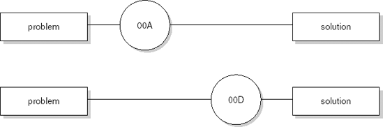
There are good reasons to distinguish OOA-type activities and OOD-type activities, as is done in Fusion, for example. During design, attention is focused on specifying how to create and destroy objects, on identifying generalizations (abstract, if necessary) of objects in order to promote reuse or maintainability, and so on. An object Publication as a generalization of Book and Journal need not be considered during analysis, since it does not increase our understanding of the domain. On the other hand, an object such as identification card may well disappear from the model during design.
Most software development organizations have accumulated a lot of experience in developing software following the traditional, function- or process-oriented style. A lot of legacy software has been developed and documented that way. As a consequence, knowledge of these methods is still required in many an organization.
Many organizations have switched to some kind of object-oriented analysis and design approach. Hard evidence of increased productivity or quality has not been determined, though. Several experiments have been done to test the effectiveness of the object-oriented paradigm, and the results do seem to indicate some deeper problems. For example, in one experiment it was tested how effective object-oriented models are as the main vehicle of communication between the typical customer and the developer (Moynihan, 1996). It was found that the traditional, functional models were easier to understand, provoked more questions and comments, gave a more holistic understanding of the business, and better helped to evaluate likely implementations. In another experiment, it was tested whether novice analysts are able to develop requirements more easily with certain methods than with others, and whether they learn to use certain methods more readily than others (Vessey and Conger, 1994). Again, the results were negative for object orientation: novice analysts were better able to apply the process-oriented method and significant learning only occurred for the process-oriented method.
In a similar vein, Arisholm and Sjøberg (2004) found that novice users have fewer problems maintaining systems that have centralized control compared to systems having delegated control. In a centralized control style, one or a few large classes are in control. These large classes coordinate the work of a lot of smaller classes. This resembles the hierarchical main-program-with-subroutines architectural style. In a delegated style, responsibilities are distributed over a larger set of classes. Proponents of object orientation usually advocate a delegated control style. It seems one needs a certain maturity to be effective with this style.
The inheritance mechanism of object orientation needs to be handled with care too, as noted in Section 12.1.6. Deep hierarchies require one to comprehend design or implementation units that may be far apart. Such designs tend to be error prone (Bieman et al., 2001) and more difficult to inspect (Dunsmore et al., 2002), because of the delocalized nature of information in them.
There may well be some truth in the observation that users do not think in objects; they think in tasks. From that point of view, use-case analysis may be seen as one way to introduce a functional view into an otherwise object-oriented approach.
A design pattern is a recurring structure of communicating components that solves a general design problem within a particular context. A design pattern differs from an architectural style in that it does not address the structure of a complete system, but only that of a few (interacting) components. Design patterns may thus be termed micro-architectures. On the other hand, a design pattern encompasses more than a single component, method or class.
The archetypal example of a design pattern is the Model-View-Controller (MVC) pattern. Interactive systems consist of computational elements as well as elements to display data and handle user input. It is considered good design practice to separate the computational elements from those that handle I/O. This separation of concerns is achieved by the MVC pattern.
MVC involves three components: the Model, the View, and the Controller. The model component encapsulates the system's data as well as the operations on those data. The model component is independent of how the data is represented or how input is done. A view component displays the data that it obtains from the model component. There can be more than one view component. Finally, each view has an associated controller component. A controller handles input actions. Such an input action may cause the controller to send a request to the model, for example to update its data, or to its view, for example to scroll.
For any given situation, the above description has to be considerably refined and made more precise. For instance, a controller may or may not depend on the state of the model. If the controller does not depend on the state of the model, there is a one-way flow of information: the controller signals an input event and notifies the model. If the controller does depend on the state of the model, information flows in the other direction as well. The latter type of dependence can be observed in most word-processing systems, for example, where menu entries are made active or inactive depending on the state of the model.
MVC was first used in the Smalltalk environment. Since then it has been applied in many applications. In various graphical user interface platforms, a variant has been applied in which the distinction between the view and the controller has been relaxed. This variant is called the Document-View pattern; see (Kruglinski, 1996).
Design patterns have a number of properties which explain what they offer, as well as why and how they do so:
A pattern addresses a recurring design problem that arises in specific design situations and presents a solution to it. Many software systems include computational elements as well as user-interface elements. For reasons of flexibility, we may wish to separate these as much as possible. MVC offers a solution to precisely this recurring problem.
A pattern must balance a set of opposing forces, i.e. characteristics of the problem that have to be dealt with in its solution. For example, in interactive applications we want to be able to present information in different ways, changes to the data must be reflected immediately in all views affected by these changes, and different 'look and feel' interfaces should not affect the application code. MVC seeks to balance all these forces.
Patterns document existing, well-proven design experience. Patterns are not invented; they evolve with experience. They reflect best practices. MVC, for example, is used in various application frameworks as well as in scores of interactive systems.
Patterns identify and specify abstractions above the level of single components. MVC has three interacting components which together solve a given problem.
Patterns provide a common vocabulary and understanding for design principles. By now, MVC has become a widely known label for a certain solution to a certain problem. We may use the term in conversation and writing much as we use terms such as 'quicksort' or 'Gauss interpolation'. Patterns thus become part of our language for describing software designs.
Patterns are a means of documentation. As with software architectures, patterns both describe and prescribe things. Descriptively, patterns offer a way to document your software, for example by simply using the pattern names in documentation. Prescriptively, pattern names give users hints as to how to extend and modify software without violating the pattern's vision. If your system employs MVC, computational aspects are strictly separated from representational aspects, and you know that this separation must be maintained during the system's evolution.
Patterns support the construction of software with defined properties. On the one hand, MVC offers a skeleton for the construction of interactive systems. MVC however also addresses certain non-functional requirements, such as flexibility and changeability of user interfaces. These non-functional requirements often constitute the major problem directly addressed by the pattern.
When describing patterns it is customary to use a schema similar to that used for describing architectural styles. The main entries of such a schema therefore are:
context: the situation giving rise to a design problem,
problem: a recurring problem arising in that situation, and
solution: a proven solution to that problem.
We illustrate this by sketching a possible application of two design patterns in a library automation system. Suppose our library system involves a central database and a number of users, some of which are based at remote sites. We wish to optimize these remote accesses, for example by using a cache. However, we do not wish to clutter the application code with code that handles such optimizations. The Proxy pattern addresses this problem. In the Proxy pattern, a client does not directly address an original. Rather, the client addresses a proxy, a representative of that original. This proxy shields the non-application specific aspects, such as optimization through a cache. The Proxy pattern can be described as in Figure 12.31.[20]
The Proxy pattern exists in many variants. The variant discussed above could be termed a Cache Proxy: emphasis is on sharing results from remote components. Other variants are the Remote Proxy (which shields network access, inter-process communication, and so on), the Protection Proxy (protection from unauthorized access) and the Firewall Proxy (protection of local clients from the outside world). Web servers typically use a Firewall Proxy pattern to protect users from the outside world.
Most users of the library system are incidental users for whom we want a friendly interface, including powerful undo facilities. On the other hand, experienced library employees want a user interface with keyboard shortcuts for most commands. Furthermore, we want to be able to log user requests for later analysis, for example to find out which authors are in demand. We want to separate these 'extras' from the actual application code. The Command Processor pattern addresses this issue. Example uses of the Command Processor pattern can, for instance, be found in user-interface toolkits. Its characteristics are given in Figure 12.32.[21]
Applications typically involve a mixture of details that pertain to different realms, such as the application domain, the representation of data to the user, the access to a remote server, and so on. If these details are mixed up in the software, the result will be difficult to comprehend and maintain.
Expert designers have learned to separate such aspects so as to increase the maintainability, flexibility, and adaptability (in short, the quality) of the systems they design. If needed, they introduce some intermediate abstract entity to bridge aspects of a solution they wish to keep separate. The Proxy and Command Processor patterns, as well as many other design patterns found in (Gamma et al., 1995) and (Buschmann et al., 1996), offer elegant and flexible solutions to precisely these divide-and-conquer type design situations.
Patterns describe common practices that have proven useful. Antipatterns describe recurring practices that have been proven to generate problems. Next to collections of patterns, people have developed collections of mistakes often made and described them as antipatterns. Knowledge of antipatterns is useful during design to prevent common pitfalls, and during evolution to improve an evolving design. In the latter case, one actually searches for antipatterns and applies a technique called refactoring to improve the design; see also Chapter 14. Descriptions of antipatterns usually include the refactoring remedy. Some well-known antipatterns are:
The God Class. In this situation, there is one central class that is in control and holds most responsibilities. It is linked to a lot of other classes that execute relatively simple tasks. It is also known as The Blob. When such a design is refactored, responsibilities are more evenly distributed. Note though that we previously observed that centralized designs are often more easily comprehended by novices.
Lava flow. At the code level, this amounts to dead code. Following the slogan 'If it ain't broken, don't touch it', obsolete code and obsolete design elements may be dragged along indefinitely.
Poltergeists. These are classes that have limited responsibilities and usually live for a short time. Their role is often just to start up other processes.
Golden Hammer. This occurs when an available solution is applied to a problem that it does not really fit ('if the only available tool is a hammer, every problem is a nail'). This antipattern is common practice when organizations feel they have to use database package X or interface toolkit Y, simply because they have a license or because their employees have deep knowledge of that technology. At the level of an individual designer, it shows up as the obsessive use of a small set of patterns.
Stovepipe. This phenomenon occurs if multiple systems are developed independently and each one uses its own set of technologies for the user interface, database, platform, and so on. Integration and cooperation then becomes difficult. Such a situation is often encountered when organizations merge or different organizations link their information systems in a chain. At a more local level, it occurs if developers or design teams reinvent the wheel.
Swiss Army Knife. This is an excessively complex class interface. It occurs when a designer wants to make a class as general and reusable as possible.
A requirements specification is developed during requirements engineering. That document serves a number of purposes. It specifies the users' requirements and as such it often has legal meaning. It is also the starting point for the design and thus serves another class of user.
The same applies to the design documentation. The description of the design serves different users, who have different needs. A proper organization of the design documentation is therefore very important.
IEEE1016 (1987) discusses guidelines for the description of a design. This standard mainly addresses the kind of information needed and its organization. For the actual description of its constituent parts, any existing design notation can be used.
(Barnard et al., 1986) distinguishes between seven user roles for the design documentation:
The project manager needs information to plan, control, and manage the project. He must be able to identify each system component and understand its purpose and function. He also needs information to make cost estimates and define work packages.
The configuration manager needs information to be able to assemble the various components into one system and to control changes.
The designer needs information about the function and use of each component and its interfaces to other components.
The programmer must know about algorithms to be used, data structures, and the kinds of interaction with other components.
The unit tester must have detailed information about components, such as algorithms used, required initialization, and data needed.
The integration tester must know about relations between components, and the function and use of the components involved.
The maintenance programmer must have an overview of the relations between components. He must know how the user requirements are realized by the various components. When changes are to be realized, he assumes the role of the designer.
In IEEE Standard 1016, the project documentation is described as an information model. The entities in this model are the components identified during the design stage. Each of these components has a number of relevant attributes, such as its name, function, and dependencies.
IEEE Standard 1016 distinguishes ten attributes. These attributes are minimally required in each project. The documentation about the design process is strongly related to the design documentation. The design process documentation includes information pertaining to, among others, the design status, alternatives that have been rejected, and revisions that have been made. It is part of configuration control, as discussed in Chapter 4. The attributes from IEEE Standard 1016 are:
Identification: the unique name of the component, for reference purposes
Type: the kind of component, such as subsystem, procedure, class, or file
Purpose: the specific purpose of the component (this will refer to the requirements specification)
Function: what the component accomplishes (for a number of components, this information occurs in the requirements specification)
Subordinates: the components of which the present entity is composed (it identifies a static is-composed-of relation between entities)
Dependencies: a description of the relationships with other components
It concerns the uses relation, see Section 12.1.5, and includes more detailed information on the nature of the interaction (including common data structures, order of execution, parameter interfaces, and so on).
Interface: a description of the interaction with other components
This concerns both the method of interaction (how to invoke an entity, how communication is achieved through parameters) and rules for the actual interaction (encompassing things such as data formats, constraints on values and the meaning of values).
Resources: the resources needed
Resources are entities external to the design, such as memory, printers, or a statistical library. This includes a discussion of how to solve possible race or deadlock situations.
Processing: a refinement of the function attribute that describes the algorithms used, initialization, and the handling of exceptions
Data: a description of the representation, use, format, and meaning of internal data.
Different users have different needs as regards design documentation. A sound organization of this documentation is needed so that each user may quickly find the information he is looking for. We may construct a matrix in which it is indicated which attributes are needed for which user role. This matrix is depicted in Table 12.6.
Table 12.6. User roles and attributes (Source: H.J. Barnard et al., A recommended practice for describing software designs: IEEE Standards Project 1016, IEEE Transactions on Software Engineering, 12(2), ©1986, IEEE.)
Attributes | User roles | ||||||
|---|---|---|---|---|---|---|---|
1 | 2 | 3 | 4 | 5 | 6 | 7 | |
Identification | x | x | x | x | x | x | x |
Type | x | x | x | x | |||
Purpose | x | x | x | ||||
Function | x | x | x | ||||
Subordinates | x | ||||||
Dependencies | x | x | x | ||||
Interface | x | x | x | x | |||
Resources | x | x | x | x | |||
Processing | x | x | |||||
Data | x | x | |||||
It is not necessarily advantageous to incorporate all attributes into one document: each user gets much more than the information needed to play his role. However, it is not necessarily advantageous to provide separate documentation for each user role: in that case, some items will occur three or four times, which is difficult to handle and complicates the maintenance of the documentation.
Table 12.7. Views on the design (Source: H.J. Barnard et al., A recommended practice for describing software designs: IEEE Standards Project 1016, IEEE Transactions on Software Engineering, 12(2), © 1986, IEEE.)
Design view | Description | Attributes | User roles |
|---|---|---|---|
Decomposition | Decomposition of the system into components | Identification, type, purpose, function, subcomponents | Project manager |
Dependencies | Relations between components and between resources | Identification, type, purpose, dependencies, resources | Configuration manager, maintenance programmer, integration tester |
Interface | How to use components | Identification, function, interfaces | Designer, integration tester |
Detail | Internal details of components | Identification, computation, data | Component tester, programmer |
In IEEE Standard 1016, the attributes are grouped into four clusters. The decomposition is made such that most users need information from only one cluster, while these clusters contain a minimum amount of superfluous information for that user. This decomposition is given in Table 12.7. It is interesting to note that each cluster has its own view on the design. Each such view gives a complete description, thereby concentrating on certain aspects of the design. This may be considered an application of the IEEE recommended practice for architectural descriptions (IEEE1471, 2000) long before that standard was developed.
The decomposition description describes the decomposition of the system into components. Using this description we may follow the hierarchical decomposition and describe the various abstraction levels.
The dependencies description gives the coupling between components. It also sums up the resources needed. We may then derive how parameters are passed and which common data is used. This information is helpful when planning changes to the system and when isolating errors or problems in resource usage.
The interface description tells us how functions are to be used. This information constitutes a contract between different designers and between designers and programmers. Precise agreements about this are especially needed in multi-person projects.
The detail description gives internal details of each component. Programmers need these details. This information is also useful when composing component tests.
Errors made at an early stage are difficult to repair and incur high costs if they are not discovered until a late stage of development. It is therefore necessary to pay extensive attention to testing and validation issues during the design stage.
The way in which the outcome of the design process can be subjected to testing strongly depends upon the way in which the design is recorded. If some formal specification technique is used (as in model-driven architecture), the resulting specification can be tested formally. It may also be possible to do static tests, such as checks for consistency. Formal specifications may sometimes be executed, which offers additional ways to test the system. Such prototypes are especially suited to testing the user interface. Users often have little idea of the possibilities to be expected and a specification-based prototype offers good opportunities for aligning users' requirements and designers' ideas.
Often, the design is stated in less formal ways, limiting the possibilities for testing to forms of reading and critiquing text, such as inspections and walkthroughs. However, such design reviews provide an extremely powerful means for assessing designs.
During the design process the system is decomposed into a number of components. We may develop test cases based on this process. These test cases may be used at a later stage, during functional testing. Conversely, the software architecture can be used to guide the testing process. A set of scenarios of typical or anticipated future usage can be used to test the quality of the software architecture.
A more comprehensive discussion of the various test techniques is given in Chapter 13.
Just like designing a house, designing software is an activity which demands creativity and a fair dose of craftsmanship. The quality of the designer is of paramount importance in this process. Mediocre designers will not deliver excellent designs.
The essence of the design process is that the system is decomposed into parts that each have less complexity than the whole. Some form of abstraction is always used in this process. We have identified several guiding principles for the decomposition of a system into components. These principles result in the following desirable properties for the outcome of the design process, a set of components with mutual dependencies:
Components should be internally cohesive, i.e. the constituents of a component should 'belong together' and 'be friends'. By identifying different levels of cohesion, a qualitative notion of component cohesion is obtained.
The interfaces between components should be as 'thin' as possible. Again, various levels of component coupling have been identified, allowing for an assessment of mutual dependencies between components.
Each component should hide one secret. Information hiding is a powerful design principle, whereby each component is characterized by a secret which it hides from its environment. Abstract data types are a prime example of the application of this principle.
The structure of the system, depicted as a graph whose nodes and edges denote components and dependencies between components, respectively, should have a simple and regular shape. The most-constrained form of this graph is a tree. In a less-constrained form the graph is acyclic, in which case the set of components can be split into a number of distinct layers of abstraction.
Abstraction is central to all of these features. In a properly designed system, we should be able to concentrate on the relevant issues and ignore the irrelevant ones. This is an essential prerequisite for comprehending a system, for implementing parts of it successfully without having to consider design decisions made elsewhere, and for implementing changes locally, thus allowing for a smooth evolution of the system.
The above features are highly interrelated and reinforce one another. Information hiding results in components with high cohesion and low coupling. Cohesion and coupling are dual characteristics. A clear separation of concerns results in a neat design structure.
We have discussed several measures for quantifying properties of a design. The most extensive research in this area concerns complexity metrics. These complexity metrics concern both attributes of individual components (called intra-component attributes) and attributes of a set of components (called intercomponent attributes).
A word of caution is needed, though. Software complexity is a very illusive notion, which cannot be captured in a few simple numbers. Different complexity metrics measure along different dimensions of what is perceived as complexity. Also, large values for any such metric do not necessarily imply a bad design. There may be good reasons to incorporate certain complex matters into one component.
A judicious and knowledgeable use of multiple design metrics is a powerful tool in the hands of the craftsman. Thoughtless application, however, will not help. To paraphrase Gunning, the inventor of the fog index (a popular readability measure for natural language prose): design metrics can cause harm in misuse.
There exist a great many design methods. They consist of a number of guidelines, heuristics, and procedures on how to approach designing a system, and notations to express the result of that process. Design methods differ considerably in their prescriptiveness, formality of notation, scope of application, and extent of incorporation in a more general development paradigm. Several tentative efforts have been made to compare design methods along different dimensions.
We discussed four design methods in this chapter:
functional decomposition,
data flow design,
data structure design, and
object-oriented design.
The first three design methods have been around longest. Object-oriented analysis and design came later, and this is now the most widely used approach, partly caused also by the popularity of the notations of UML and its associated tools and full-scale development methods, such as RUP.
Proponents of object-oriented methods have claimed a number of advantages of the object-oriented approach over the more traditional, function-oriented, approaches to design:
The object-oriented approach is more natural. It fits the way we view the world around us. The concepts that show up in the analysis model have a direct counterpart in the UoD being modeled, thus providing a direct link between the model and the world being modeled. This makes it easier for the client to comprehend the model and discuss it with the analyst.
The object-oriented approach focuses on structuring the problem rather than any particular solution to it. This point is closely related to the previous one. In designs based on the functional paradigm, the components tend to correspond to parts of a solution to the problem. It may not be easy to relate these components to the original problem. The result of an object-oriented analysis and design is a hierarchy of objects with their associated attributes which still resembles the structure of the problem space.
The object-oriented approach provides for a smoother transition from requirements analysis to design to code. In our discussion of the object-oriented approach, it is often difficult to strictly separate UoD modeling aspects from design aspects. The object hierarchy that results from this process can be directly mapped onto the class hierarchy of the implementation (provided the implementation language is also object-oriented). The attributes of objects become encapsulated by services provided by the objects in the implementation.
The object-oriented approach leads to more flexible systems that are easier to adapt and change. Because the real-world objects have a direct counterpart in the implementation, it becomes easy to link change requests to the corresponding program components. Through the inheritance mechanism, changes can often be realized by adding another specialized object rather than through tinkering with the code. For example, if we wish to extend our system dealing with furniture by adding another type of chair, say armchair, we do so by defining a new object
ArmChair, together with its own set of attributes, as another specialization ofChair.The object-oriented approach promotes reuse by focusing on the identification of real-world objects from the application domain. In contrast, more traditional approaches focus on identifying functions. In an evolving world, objects tend to be stable, while functions tend to change. For instance, in an office environment the functions performed are likely to change with time, but there will always be letters, folders, and so on. Thus, an object-oriented design is less susceptible to changes in the world being modeled.
The inheritance mechanism adds to reusability. New objects can be created as specializations of existing objects, inheriting attributes from the existing objects. At the implementation level, this kind of reuse is accomplished through code sharing. The availability of extensive class libraries contributes to this type of code reuse.
Objects in an object-oriented design encapsulate abstract data types. As such, an object-oriented design potentially has all the right properties (such as information hiding, abstraction, high cohesion, and low coupling).
The object-oriented approach, however, does not by definition result in a good design. It is a bit too naive to expect that the identification of domain-specific entities is all there is to good design. The following issues must be kept in mind:
There are other objects besides the ones induced by domain concepts. Objects that have to do with system issues such as memory management or error recovery do not naturally evolve from the modeling of the UoD. Likewise, 'hypothetical' objects that capture implicit knowledge from the application domain may be difficult to identify.
The separation of concerns that results from the encapsulation of both state and behavior into one component need not be the one that is most desirable. For example, for many an object it might be necessary to be able to present some image of that object to the user. In a straightforward application of the object-oriented method, this would result in each object defining its own ways for doing so. This, however, is against good practices of system design, where we generally try to isolate the user interface from the computational parts. A clearly identifiable user interface component adds to consistency and flexibility.
With objects, we also have to consider the uses relation. An object uses another object if it requests a service from that other object. It does so by sending a message. The bottom-up construction of a collection of objects may result in a rather loosely-coupled set, in which objects freely send messages to other objects. With a nod at the term 'spaghetti code' (denoting overly complex control patterns in programs), this is known as the ravioli problem (or antipattern). If objects have a complicated usage pattern, it is difficult to view one object without having to consider many others as well.
A design pattern is a structure of communicating components that solves a general design problem within a particular context. A design pattern thus encompasses more than a single component. It involves some, usually 2–5, communicating components which together solve a problem. The problem that the pattern solves is a general, recurring one, which can be characterized by the context in which it arises. A design pattern differs from an architectural style in that it does not address the structure of a complete system, but only that of a few (interacting) components. Design patterns may thus be termed micro-architectures. Not surprisingly, the good things about design patterns are essentially the same as those listed for software architectures in Chapter 11.
Design patterns describe best practice. They represent the collective experience of some of the most experienced and successful software designers. Likewise, antipatterns describe widely shared bad practices. The description of both patterns and antipatterns, as found in textbooks, is the result of endless carving and smoothing. Some are the outcome of writers' workshops, a format commonly used to review literature, suggesting that we should review software literature with a profoundness like that used to review poetry (as a consequence, these writers' workshops are also known as workers' write shops).
The distinction between the notions of 'software architecture' and 'design pattern' is by no means sharp. Some authors for example use the term 'architectural pattern' to denote the architectural styles we discussed in Section 11.4. The notions of 'application framework' and 'idiom' are generally used to denote a software architecture and a design pattern, respectively, at a more concrete, implementation-specific level. But again, the distinction is not sharp.
Finally, the design itself must be documented. IEEE Standard 1016 may serve as a guideline for this documentation. It lists a number of attributes for each component of the design. These attributes may be clustered into four groups, each of which represents a certain view of the design. This resembles the way IEEE Standard 1471 advocates documenting a software architecture.
Unfortunately, the design documentation typically describes only the design result and not the process that led to that particular result. Yet, information about choices made, alternatives rejected, and deliberations on the design decisions is a valuable additional source of information when a design is to be implemented, assessed, or changed.
(Budgen, 2003) is a good textbook on software design. I found the 'software as a wicked problem' analogy in that text. (Bergland and Gordon, 1981) and (Freeman and Wasserman, 1983) are compilations of seminal articles on software design. For an interesting discussion on the 'Scandinavian' approach to system development, see (Floyd et al., 1989) or (CACM, 1993a). Wieringa (1998) provides an extensive survey of both classical and object-oriented design methods and their notations.
The classic text on structured analysis and design is (Yourdon and Constantine, 1975). Other names associated with the development of SA/SD are DeMarco (1979) and Gane and Sarson (1979).
For a full exposition of JSP, the reader is referred to (Jackson, 1975) or (King, 1988). JSP is very similar to a method developed by J.-D. Warnier in France at about the same time (Warnier, 1974). The latter is known as Logical Construction of Programs (LCP) or the Warnier-Orr method, after Ken Orr who was instrumental in the translation of Warnier's work. For a full exposition of JSD, see (Jackson, 1983), (Cameron, 1989) or (Sutcliffe, 1988). The graphical notations used in this chapter are those of (Sutcliffe, 1988).
Booch's method for object-oriented analysis and design is discussed in (Booch, 1994). Fusion is described in (Coleman et al., 1994). Updates to this 1994 version can be found in (Coleman, 1996). RUP is discussed in (Kruchten, 2003). A critical discussion of the differences and similarities between object-oriented analysis and object-oriented design is given in (Davis, 1995) and (Hødalsvik and Sindre, 1993).
Fenton and Pfleeger (1996) present a rigorous approach to the topic of software metrics. The authors explain the essentials of measurement theory and illustrate them using a number of proposed metrics (including those for complexity, quality assessment, and cost estimation).
Cohesion and coupling were introduced in (Yourdon and Constantine, 1975). Efforts to objectify these notions can be found in (Offutt et al., 1993), (Patel et al., 1992) and (Xia, 2000). Darcy (2005) describes empirical studies to validate the importance of weak coupling and strong cohesion.
Halstead's method, 'software science', is described in (Halstead, 1977) and (Fitzsimmons and Love, 1978). Positive evidence of its validity is reported in (Curtis et al., 1979) and (Elshoff, 1976). A good overview of the criticism of this method (as well as McCabe's cyclomatic complexity and Henri and Kafura's information flow metric) is given in (Shepperd and Ince, 1993). McCabe's cyclomatic complexity is introduced in (McCabe, 1976). In most discussions of this metric, the wrong formula is used; see Exercise 24 or (Henderson Sellers, 1992). Discussions in favor of using a (cyclomatic) complexity density metric can be found in (Mata-Toledo and Gustafson, 1992) and (Hops and Sherif, 1995).
Definitions of the object-oriented metrics introduced in Section 12.1.6 can be found in (Chidamber and Kemerer, 1994). A critical assessment of these metrics is given in (Hitz and Montazeri, 1996) and (Churcher and Shepperd, 1995). To meet some of this criticism, we have adopted the definition of LCOM suggested in (Li and Henry, 1993). Experiments to validate the Chidamber-Kemerer metrics suite are reported in (Succi et al., 2003), (Darcy and Kemerer, 2005) and (Gyimóthy et al., 2005).
Design patterns have their origin in the work of Cunningham and Beck, who developed patterns for user interfaces in Smalltalk, such as 'no more than three panes per window' (Power and Weiss, 1987, p. 16). MVC was first used in the Smalltalk environment (Krasner and Pope, 1988). Since that time, the topic has drawn a lot of attention, especially in object-oriented circles. A major collection of design patterns was published by the 'Gang of Four' (Gamma et al., 1995). Another good collection of design patterns can be found in (Buschmann et al., 1996). The latter text has a somewhat less object-oriented perspective than (Gamma et al., 1995). (Brown et al., 1998) describe a collection of well-known antipatterns. Since 1994, there has been an annual conference on pattern languages of programming (PLOP). The format for describing patterns has not only been used for design patterns; there are also collections of analysis patterns, process patterns, test patterns, etc.
What is the difference between procedural abstraction and data abstraction?
List and explain Yourdon and Constantine's seven levels of cohesion.
Explain the notions cohesion and coupling.
In what sense are the various notions of coupling technology-dependent?
What is the essence of information hiding?
Give an outline of Halstead's software science.
Determine the cyclomatic complexity of the following program:
no_6 = true; sum = 0;
for(i = 1; i<no_of_courses; i++) {if(grade[i]<7) no_6 = false; sum = sum + grade[i]; }; average = sum / no_of_courses;if((average ≥ 8) && (no_6)) System.out.println("with distinction");Would the cyclomatic complexity be any different if the last
ifstatement were written as follows:if(average ≥ 8) {if(no_6) System.out.println("with distinction"); }Does this concur with your own ideas of a control complexity measure, i.e. does it fulfill the representation condition?
Give the formula and a rationale for the information flow complexity metric.
Is cyclomatic complexity a good indicator of system complexity?
Draw the call graphs for a nontrivial program you have written and determine its tree impurity. Does the number obtained agree with our intuitive idea about the 'quality' of the decomposition?
Compute Henri and Kafura's information flow metric for the design of two systems you have been involved in. Do these numbers agree with our intuitive understanding?
Why is the depth of a class in the inheritance tree (DIT) a useful metric to consider when assessing the quality of an object-oriented system?
What does response for a class (RFC) measure?
How does the Law of Demeter relate to the maintainability of object-oriented systems?
Discuss the relative merits and drawbacks of deep and narrow versus wide and shallow inheritance trees.
What is functional decomposition?
Give a global sketch of the data flow design method.
Explain what a structure clash is in JSP.
What is the main difference between problem-oriented and product-oriented design methods?
Discuss the general flavor of RUP's analysis and design workflow.
What are the differences between object-oriented design and the simple application of the information-hiding principle?
What are the properties of a design pattern?
Hint: consider the following program:
beginifAthenBelseCendif; call P; print("done")end;procedureP;beginifXthenYelseZendifendP;Draw the flow graph for this program as well as for the program obtained by substituting the body of procedure
Pinline. Determine the cyclomatic complexity of both variants, using both formulae. See also (Henderson Sellers, 1992).
functional decomposition,
data flow design,
design based on data structures, and
object-oriented design
for the design of each of:
a compiler,
a patient-monitoring system, and
a stock-control system.
m(G) = 0 if and only if G is a tree;
m(G1) > m(G2) if G1 differs from G2 only by the insertion of an extra arc;
For i = 1, 2 let Ai denote the number of arcs in Gi and Ni the number of nodes in Gi. Then if N1 > N2 and A1 − N1 + 1 = A2 − N2 + 1, then m(G1) < m(G2).
For all graphs G, m(G) ≤ m(KN) = 1 where N = number of nodes of G and KN is the (undirected) complete graph of N nodes.
Give an intuitive rationale for these properties. Show that the tree impurity metric discussed in Section 12.1.5 has these properties.
[14] Obviously, an even more important property of a design is that the corresponding system should perform the required tasks in the specified way. To this end, the design should be validated against the requirements.
[15] The number of linearly independent paths is related to the cyclomatic number of a graph, which is why this is called the 'cyclomatic complexity'.
[16] We assume that the graph is connected, i.e. that there is a path between each pair of nodes if we ignore the direction of the arrows that link nodes. This assumption is reasonable, since otherwise the graph can be split into two or more disjoint graphs between which there is no information flow. These disjoint graphs then correspond to independent components.
[17] The Law of Demeter is a generally accepted design heuristic for object-oriented systems. It says that the methods of a class should depend only on the top-level structure of their own class. More specifically, in the context of a class C with method M, M should only send messages to:
the parameters of C, or
the state variables of C, or
C itself.
[18] We do the same when turning a free tree into an oriented tree. A free tree has no root. By selecting one node of the tree as the root, the parent-child relations are brought about.
[19] For simplicity's sake, we have assumed that the input is already sorted by author.
[20] See (Buschmann et al., 1996, pp. 263–75) for a more elaborate description.
[21] see (Buschmann et al., 1996, pp. 277–90) for a more elaborate description.