
Chapter 9
Digital recording and editing systems
This chapter describes digital audio recording systems and the principles of digital audio editing.
Digital tape recording
There are still a number of dedicated digital tape recording formats in existence, although they are being superseded by computer-based products that use removable disks or other mass storage media. Tape has a relatively slow access time, because it is a linear storage medium. However, a dedicated tape format can easily be interchanged between recorders, provided that another machine operating to the same standard can be found. Disks, on the other hand, come in a very wide variety of sizes and formats, and even if the disk fits a particular drive it may not be possible to access the audio files thereon, owing to the multiplicity of levels at which compatibility must exist between systems before interchange can take place.
Background to digital tape recording
When commercial digital audio recording systems were first introduced in the 1970s and early 1980s it was necessary to employ recorders with sufficient bandwidth for the high data rates involved (a machine capable of handling bandwidths of a few megahertz was required). Analogue audio tape recorders were out of the question because their bandwidths extended only up to around 35 kHz at best, so video tape recorders (VTRs) were often utilised because of their wide recording bandwidth. PCM adaptors converted digital audio data into a waveform which resembled a television waveform, suitable for recording on to a VTR. The Denon company of Japan developed such a system in partnership with the NHK broadcasting organisation and they released the world’s first PCM recording on to LP in 1971. In the early 1980s, devices such as Sony’s PCM-F1 became available at modest prices, allowing 16 bit, 44.1 kHz digital audio to be recorded on to a consumer VTR, resulting in widespread proliferation of stereo digital recording. Dedicated open-reel digital recorders using stationary heads were also developed (see Fact File 9.1). High density tape formulations were then manufactured for digital use, and this, combined with new channel codes (see below), improvements in error correction and better head design, led to the use of a relatively low number of tracks per channel, or even single-track recording of a given digital signal, combined with playing speeds of 15 or 30 inches per second. Dedicated rotary-head systems, not based on a VTR, were also developed – the R-DAT format being the most well known.
Digital recording tape is thinner (27.5 microns) than that used for analogue recordings; long playing times can be accommodated on a reel, but also thin tape contacts the machine’s heads more intimately than does standard 50 micron thickness tape which tends to be stiffer. Intimate contact is essential for reliable recording and replay of such a densely packed and high bandwidth signal.
Fact file 9.1 Rotary and stationary heads
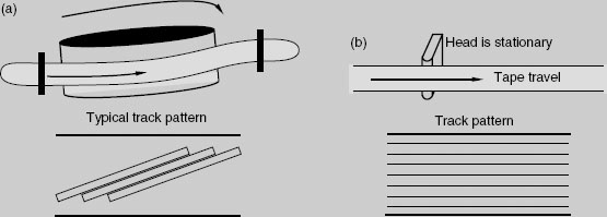
There are two fundamental mechanisms for the recording of digital audio on tape, one which uses a relatively low linear tape speed and a quickly rotating head, and one which uses a fast linear tape speed and a stationary head. In the rotary-head system the head either describes tracks almost perpendicular to the direction of tape travel, or it describes tracks which are almost in the same plane as the tape travel. The former is known as transverse scanning, and the latter is known as helical scanning, as shown in (a). Transverse scanning uses more tape when compared with helical scanning. It is not common for digital tape recording to use the transverse scanning method. The reason for using a rotary head is to achieve a high head-to-tape speed, since it is this which governs the available bandwidth. Rotary-head recordings cannot easily be splice-edited because of the track pattern, but they can be electronically edited using at least two machines.
Stationary heads allow the design of tape machines that are very similar in many respects to analogue transports. With stationary-head recording it is possible to record a number of narrow tracks in parallel across the width of the tape, as shown in (b). Tape speed can be traded off against the number of parallel tracks used for each audio channel, since the required data rate can be made up by a combination of recordings made on separate tracks. This approach was used in the DASH format, where the tape speed could be 30 ips (76 cm s−1) using one track per channel, 15 ips using two tracks per channel, or 7.5 ips using four tracks per channel.
Channel coding for dedicated tape formats
Since ‘raw’ binary data is normally unsuitable for recording directly by dedicated digital recording systems, a ‘channel code’ is used which matches the data to the characteristics of the recording system, uses storage space efficiently, and makes the data easy to recover on replay. A wide range of channel codes exists, each with characteristics designed for a specific purpose. The channel code converts a pattern of binary data into a different pattern of transitions in the recording or transmission medium. It is another stage of modulation, in effect. Thus the pattern of bumps in the optical surface of a CD bears little resemblance to the original audio data, and the pattern of magnetic fiux transitions on a DAT cassette would be similarly different. Given the correct code book, one could work out what audio data was represented by a given pattern from either of these systems.
Many channel codes are designed for a low DC content (in other words, the data is coded so as to spend, on average, half of the time in one state and half in the other) in cases where signals must be coupled by transformers (see ‘Transformers’, Chapter 12), and others may be designed for narrow bandwidth or a limited high-frequency content. Certain codes are designed specifically for very high density recording, and may have a low clock content with the possibility for long runs in one binary state or the other without a transition. Channel coding involves the incorporation of the data to be recorded with a clock signal, such that there is a sufficient clock content to allow the data and clock to be recovered on replay (see Fact File 9.2). Channel codes vary as to their robustness in the face of distortion, noise and timing errors in the recording channel.
Some examples of channel codes used in audio systems are shown in Figure 9.1. FM is the simplest, being an example of binary frequency modulation. It is otherwise known as ‘bi-phase mark’, one of the Manchester codes, and is the channel code used by SMPTE/EBU timecode (see Chapter 15). MFM and Miller-squared are more efficient in terms of recording density. MFM is more efficient than FM because it eliminates the transitions between successive ones, only leaving them between successive zeros. Miller2 eliminates the DC content present in MFM by removing the transition for the last one in an even number of successive ones.
Group codes, such as that used in the Compact Disc and R-DAT, involve the coding of patterns of bits from the original audio data into new codes with more suitable characteristics, using a look-up table or ‘code book’ to keep track of the relationship between recorded and original codes. This has clear parallels with coding as used in intelligence operations, in which the recipient of a message requires the code book to be able to understand the message. CD uses a method known as 8-to-14 modulation, in which 16 bit audio sample words are each split into two 8 bit words, after which a code book is used to generate a new 14 bit word for each of the 256 possible combinations of 8 bits. Since there are many more words possible with 14 bits than with 8, it is possible to choose those which have appropriate characteristics for the CD recording channel. In this case, it is those words which have no more than 11 consecutive bits in the same state, and no less than three. This limits the bandwidth of the recorded data, and makes it suitable for the optical pick-up process, whilst retaining the necessary clock content.
Fact file 9.2 Data recovery
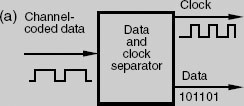
Channel-coded data must be decoded on replay, but first the audio data must be separated from the clock information which was combined with it before recording. This process is known as data and sync separation, as shown in (a).
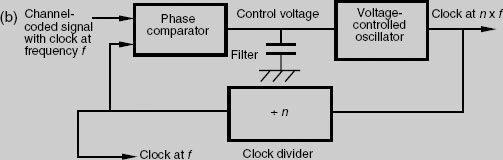
It is normal to use a phase-locked loop for the purpose of regenerating the clock signal from the replayed data, as shown in (b), this being based around a voltage-controlled oscillator (VCO) which runs at some multiple of the off-tape clock frequency. A phase comparator compares the relative phases of the divided VCO output and the clock data off tape, producing a voltage proportional to the error which controls the frequency of the VCO. With suitable damping, the phase-locked oscillator will ‘flywheel’ over short losses or irregularities of the off-tape clock.
Recorded data is usually interspersed with synchronising patterns in order to give the PLL in the data separator a regular reference in the absence of regular dock data from the encoded audio signal, since many channel codes have long runs without a transition.
Even if the off-tape data and clock have timing irregularities, such as might manifest themselves as ‘wow’ and ‘flutter’ in analogue reproducers (see ‘Wow and flutter’, Appendix 1), these can be removed in digital systems. The erratic data (from tape or disk, for example) is written into a short-term solid state memory (RAM) and read out again a fraction of a second later under control of a crystal clock (which has an exceptionally stable frequency), as shown in (c). Provided that the average rate of input to the buffer is the same as the average rate of output, and the buffer is of sufficient size to soak up short-term irregularities in timing, the buffer will not overflow or become empty.
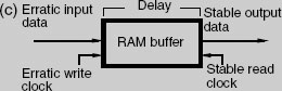
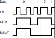
Figure 9.1 Examples of three channel codes used in digital recording. Miller-squared is the most efficient of those shown since it involves the smallest number of transitions for the given data sequence
Error correction
There are two stages to the error correction process used in digital tape recording systems. Firstly, the error must be detected, and then it must be corrected. If it cannot be corrected then it must be concealed. In order for the error to be detected it is necessary to build in certain protection mechanisms.
Two principal types of error exist: the burst error and the random error. Burst errors result in the loss of many successive samples and may be due to major momentary signal loss, such as might occur at a tape drop-out or at an instant of impulsive interference such as an electrical spike induced in a cable or piece of dirt on the surface of a CD. Burst error correction capability is usually quoted as the number of consecutive samples which may be corrected perfectly. Random errors result in the loss of single samples in randomly located positions, and are more likely to be the result of noise or poor signal quality. Random error rates are normally quoted as an average rate, for example: 1 in 106. Error correction systems must be able to cope with the occurrence of both burst and random errors in close proximity.
Audio data is normally interleaved before recording, which means that the order of samples is shuffled (as shown conceptually in Figure 9.2). Samples that had been adjacent in real time are now separated from each other on the tape. The benefit of this is that a burst error, which destroys consecutive samples on tape, will result in a collection of single-sample errors in between good samples when the data is deinterleaved, allowing for the error to be concealed. A common process, associated with interleaving, is the separation of odd and even samples by a delay. The greater the interleave delay, the longer the burst error that can be handled. A common example of this is found in the DASH tape format (an open-reel digital recording format), and involves delaying odd samples so that they are separated from even samples by 2448 samples, as well as reordering groups of odd and even samples within themselves.
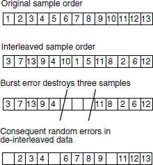
Figure 9.2 Interleaving is used in digital recording and broadcasting systems to rearrange the original order of samples for storage or transmission. This can have the effect of converting burst errors into random errors when the samples are deinterleaved
Redundant data is also added before recording. Redundancy, in simple terms, involves the recording of data in more than one form or place. A simple example of the use of redundancy is found in the twin-DASH format, in which all audio data is recorded twice. On a second pair of tracks (handling the duplicated data), the odd–even sequence of data is reversed to become even–odd. Firstly, this results in double protection against errors, and secondly, it allows for perfect correction at a splice, since two burst errors will be produced by the splice, one in each set of tracks. Because of the reversed odd–even order in the second set of tracks, uncorrupted odd data can be used from one set of tracks, and uncorrupted even data from the other set, obviating the need for interpolation (see Fact File 9.3).
Cyclic redundancy check (CRC) codes, calculated from the original data and recorded along with that data, are used in many systems to detect the presence and position of errors on replay. Complex mathematical procedures are also used to form codewords from audio data which allow for both burst and random errors to be corrected perfectly up to a given limit. Reed–Solomon encoding is another powerful system which is used to protect digital recordings against errors, but it is beyond the scope of this book to cover these codes in detail.
Digital tape formats
There have been a number of commercial recording formats over the last 20 years, and only a brief summary will be given here of the most common.
Sony’s PCM-1610 and PCM-1630 adaptors dominated the CD-mastering market for a number of years, although by today’s standards they used a fairly basic recording format and relied on 60 Hz/525 line U-matic cassette VTRs (Figure 9.3). The system operated at a sampling rate of 44.1 kHz and used 16 bit quantisation, being designed specifically for the making of tapes to be turned into CDs. Recordings made in this format could be electronically edited using the Sony DAE3000 editing system, and the playing time of tapes ran up to 75 minutes using a tape specially developed for digital audio use.
The R-DAT or DAT format is a small stereo, rotary-head, cassette-based format offering a range of sampling rates and recording times, including the professional rates of 44.1 and 48 kHz. Originally, consumer machines operated at 48 kHz to avoid the possibility for digital copying of CDs, but professional versions became available which would record at either 44.1 or 48 kHz. Consumer machines will record at 44.1 kHz, but usually only via the digital inputs. DAT is a 16 bit format, but has a non-linearly encoded long-play mode as well, sampled at 32 kHz. Truly professional designs offering editing facilities, external sync and IEC-standard timecode have also been developed. The format became exceptionally popular with professionals owing to its low cost, high performance, portability and convenience. Various non-standard modifications were introduced, including a 96 kHz sampling rate machine and adaptors enabling the storage of 20 bit audio on such a high sampling rate machine (sacrificing the high sampling rate for more bits). The IEC timecode standard for R-DAT was devised in 1990. It allows for SMPTE/EBU timecode of any frame rate to be converted into the internal DAT ‘running-time’ code, and then converted back into any SMPTE/EBU frame rate on replay. A typical machine is pictured in Figure 9.4.
Fact file 9.3 Error handling
True correction
Up to a certain random error rate or burst error duration an error correction system will be able to reconstitute erroneous samples perfectly. Such corrected samples are indistinguishable from the originals, and sound quality will not be affected. Such errors are often signalled by green lights showing ‘CRC’ failure or ‘Parity’ failure.
Interpolation
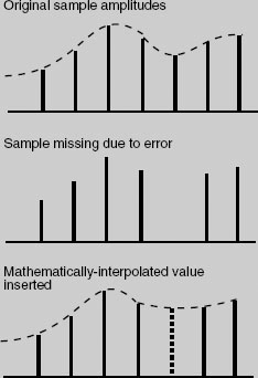
When the error rate exceeds the limits for perfect correction, an error correction system may move to a process involving interpolation between good samples to arrive at a value for a missing sample (as shown in the diagram). The interpolated value is the mathematical average of the foregoing and succeeding samples, which may or may not be correct. This process is also known as concealment or averaging, and the audible effect is not unpleasant, although it will result in a temporary reduction in audio bandwidth. Interpolation is usually signalled by an orange indicator to show that the error condition is fairly serious. In most cases the duration of such concealment is very short, but prolonged bouts of concealment should be viewed warily, since sound quality will be affected. This will usually point to a problem such as dirty heads or a misaligned transport, and action should be taken.
Hold
In extreme cases, where even interpolation is impossible (when there are not two good samples either side of the bad one), a system may ‘hold’. In other words, it will repeat the last correct sample value. The audible effect of this will not be marked in isolated cases, but is still a severe condition. Most systems will not hold for more than a few samples before muting. Hold is normally indicated by a red light.
Mute
When an error correction system is completely overwhelmed it will usually effect a mute on the audio output of the system. The duration of this mute may be varied by the user in some systems. The alternative to muting is to hear the output, regardless of the error. Depending on the severity of the error, it may sound like a small ‘spit’, click, or even a more severe breakup of the sound. In some cases this may be preferable to muting.
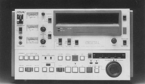
Figure 9.3 Sony DMR-4000 digital master recorder. (Courtesy of Sony Broadcast and Professional Europe)
The Nagra-D recorder (Figure 9.5) was designed as a digital replacement for the world-famous Nagra analogue recorders, and as such was intended for professional use in field recording and studios. The format was designed to have considerable commonality with the audio format used in D1- and D2-format digital VTRs, having rotary heads, although it uses open reels for operational convenience. Allowing for 20–24 bits of audio resolution, the Nagra-D format was appropriate for use with high resolution convertors. The error correction and recording density used in this format were designed to make recordings exceptionally robust, and recording time could be up to 6 hours on a 7 inch (18 cm) reel, in two-track mode. The format is also designed for operation in a four-track mode at twice the stereo tape speed, such that in stereo the tape travels at 4.75 cm s-1, and in four track at 9.525 cm s−1.
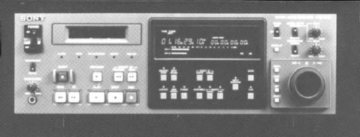
Figure 9.4 Sony PCM-7030 professional DAT machine. (Courtesy of Sony Broadcast and Professional Europe)
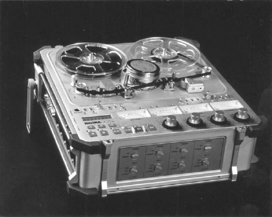
Figure 9.5 Nagra-D open-reel digital tape recorder. (Courtesy of Sound PR)
The DASH (Digital Audio Stationary Head) format consisted of a whole family of open-reel stationary-head recording formats from two tracks up to 48 tracks. DASH-format machines operated at 44.1 kHz or 48 kHz rates (and sometimes optionally at 44.056 kHz), and they allowed varispeed ±12.5 per cent. They were designed to allow gapless punch-in and punch-out, splice editing, electronic editing and easy synchronisation. Multitrack DASH machines (an example is shown in Figure 9.6) gained wide acceptance in studios, but the stereo machines did not. Later developments resulted in DASH multitracks capable of storing 24 bit audio instead of the original 16 bits.
In more recent years budget modular multitrack formats were introduced. Most of these were based on eight-track cassettes using rotary head transports borrowed from consumer video technology. The most widely used were the DA-88 format (based on Hi-8 cassettes) and the ADAT format (based on VHS cassettes). These offered most of the features of open reel machines and a number of them could be synchronised to expand the channel capacity. An example is shown in Figure 9.7.
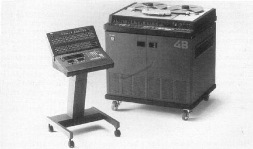
Figure 9.6 An open-reel digital multitrack recorder: the Sony PCM-3348. (Courtesy of Sony Broadcast and Professional Europe)
Performance and alignment
Crosstalk between the tracks of a digital recorder is virtually absent, and this frees the engineer from the need to allocate tracks carefully. For example, with an analogue multitrack machine one tends to record vocals on tracks, which are physically far away on the tape from, say, drum tracks, since crosstalk from the latter can easily be audible. Unused tracks will often be used to form an extended guard band to separate, say, an electric guitar track or timecode track from a vocal. None of this is necessary with a digital multitrack recorder. Other recording artefacts commonly encountered with analogue recordings, such as wow and flutter, are also absent on digital machines.
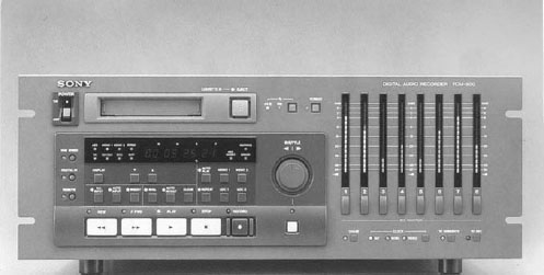
Figure 9.7 A modular digital multitrack machine, Sony PCM-800. (Courtesy of Sony Broadcast and Professional Europe)
Digital tape machines require at least as much care and maintenance as do their analogue counterparts. In fact, the analogue machine can be monitored for slight deterioration in performance rather more easily than can the digital. Slight frequency response fall-off, for example, due to, say, head wear or azimuth misalignment, can quickly be checked for and spotted using a test tape on an analogue machine. Misalignment of a digital machine, however, will cause two types of problem, neither of which is easily spotted unless careful checks are regularly carried out. First, a machine’s transport may be misaligned such that although tapes recorded on it will replay satisfactorily on the same machine, another correctly aligned machine may well not be able to obtain sufficient data from the tape to reconstitute the signal adequately. Error correction systems will be working too hard and drop-outs will occur. Second, digital recording tends to work without noticeable performance deterioration until things get so bad that drop-outs occur. There is little warning of catastrophic drop-outs, although the regularity of errors is an excellent means of telling how close to the edge a system is in terms of random errors. If a recorder has error status indication, these can be used to tell the prevailing state of the tape or the machine’s alignment. Different degrees of seriousness exist, as discussed in Fact File 9.3. If the machine is generating an almost constant string of CRC errors or interpolations, then this is an indication that either the tape or the machine is badly out of alignment or worn. It is therefore extremely important to check alignment often and to clean the machine’s heads using whatever means is recommended. Alignment may require specialised equipment, which dealers will usually possess.
Editing digital tape recordings
Razor blade cut-and-splice editing was possible on open-reel digital formats, and the analogue cue tracks were monitored during these operations. This was necessary because the digital tracks were generally only capable of being replayed at speeds that were no more than about 10 per cent away from normal replay speed. The analogue tracks were of low quality – rather lower than a dedicated analogue machine – but usually adequate as a cue.
A 90° butt joint was used for the splice editing of digital tape. The discontinity in the data stream caused by the splice would cause complete momentary drop-out of the digital signal if no further action were taken, so circuits were incorporated that sensed the splice and performed an electronic crossfade from one side of the splice to the other, with error concealment to minimise the audibility of the splice. It was normally advised that a 0.5 mm gap should be left at the splice so that its presence would easily be detected by the crossfade circuitry. The thin tape could easily be damaged during the cut-and-splice edit procedure. Electronic editing was far more desirable, and was the usual method.
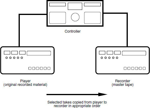
Figure 9.8 In electronic tape copy editing selected takes are copied in sequence from player to recorder with appropriate crossfades at joins
Electronic editing normally required the use of two machines plus a control unit, as shown in the example in Figure 9.8. A technique was employed whereby a finished master tape was assembled from source takes on player machines. This was a relatively slow process, as it involved real-time copying of audio from one machine to another, and modifications to the finished master were difficult. The digital editor could often store several seconds of programme in its memory and this could be replayed at normal speed or under the control of a search knob which enabled very slow to-and-fro searches to be performed in the manner of rock and roll editing on an analogue machine. Edits could be rehearsed prior to execution. When satisfactory edit points had been determined the two machines were synchronised using timecode, and the record machine switched to drop in the new section of the recording from the replay machine at the chosen moment. Here a crossfade is introduced between old and new material to smooth the join. The original source tape was left unaltered.
Disk-based systems
Once audio is in a digital form it can be handled by a computer, like any other data. The only real difference is that audio requires a high sustained data rate, substantial processing power and large amounts of storage compared with more basic data such as text. The following is an introduction to some of the technology associated with computer-based audio workstations and audio recording using computer mass storage media such as hard disks. Much more detail will be found in Desktop Audio Technology, as detailed in the Further reading list. The MIDI-based aspects of such systems are covered in Chapter 14.
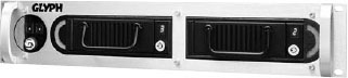
Figure 9.9 A typical removable disk drive system allowing multiple drives to be inserted or removed from the chassis at will. Frame housing multiple removable drives. (Courtesy of Glyph Technologies Inc.)
Magnetic hard disks
Magnetic hard disk drives are probably the most common form of mass storage. They have the advantage of being random-access systems – in other words any data can be accessed at random and with only a short delay. There exist both removable and fixed media disk drives, but in almost all cases the fixed media drives have a higher performance than removable media drives. This is because the design tolerances can be made much finer when the drive does not have to cope with removable media, allowing higher data storage densities to be achieved. Some disk drives have completely removable drive cartridges containing the surfaces and mechanism, enabling hard disk drives to be swapped between systems for easy project management (an example is shown in Figure 9.9).
The general structure of a hard disk drive is shown in Figure 9.10. It consists of a motor connected to a drive mechanism that causes one or more disk surfaces to rotate at anything from a few hundred to many thousands of revolutions per minute. This rotation may either remain constant or may stop and start, and it may either be at a constant rate or a variable rate, depending on the drive. One or more heads are mounted on a positioning mechanism which can move the head across the surface of the disk to access particular points, under the control of hardware and software called a disk controller. The heads read data from and write data to the disk surface by whatever means the drive employs.
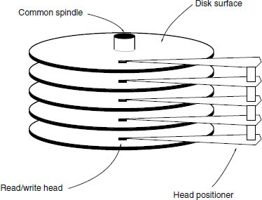
Figure 9.10 The general mechanical structure of a disk drive
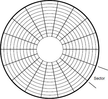
Figure 9.11 Disk formatting divides the storage area into tracks and sectors
The disk surface is normally divided up into tracks and sectors, not physically but by means of ‘soft’ formatting (see Figure 9.11). Low-level formatting places logical markers, which indicate block boundaries, amongst other processes. On most hard disks the tracks are arranged as a series of concentric rings, but with some optical discs there is a continuous spiral track.
Disk drives look after their own channel coding, error detection and correction so there is no need for system designers to devise dedicated audio processes for disk-based recording systems. The formatted capacity of a disk drive is all available for the storage of ‘raw’ audio data, with no additional overhead required for redundancy and error checking codes. ‘Bad blocks’ are mapped out during the formatting of a disk, and not used for data storage. If a disk drive detects an error when reading a block of data it will attempt to read it again. If this fails then an error is normally generated and the file cannot be accessed, requiring the user to resort to one of the many file recovery packages on the market. Disk-based audio systems do not resort to error interpolation or sample hold operations, unlike tape recorders. Replay is normally either correct or not possible.
RAID arrays enable disk drives to be combined in various ways as described in Fact File 9.4.
Fact File 9.4 RAID arrays
Hard disk drives can be combined in various ways to improve either data integrity or data throughput. RAID stands for Redundant Array of Inexpensive Disks, and is a means of linking ordinary disk drives under one controller so that they form an array of data storage space. A RAID array can be treated as a single volume by a host computer. There are a number of levels of RAID array, each of which is designed for a slightly different purpose, as summarised in the table.
RAID level | Features |
0 | Data blocks split alternately between a pair of disks, but no redundancy so actually less reliable than a single disk. Transfer rate is higher than a single disk. Can improve access times by intelligent controller positioning of heads so that next block is ready more quickly |
1 | Offers disk mirroring. Data from one disk is automatically duplicated on another. A form of real-time backup |
2 | Uses bit interleaving to spread the bits of each data word across the disks, so that, say, eight disks each hold one bit of each word, with additional disks carrying error protection data. Non-synchronous head positioning. Slow to read data, and designed for mainframe computers |
3 | Similar to level 2, but synchronises heads on all drives, and ensures that only one drive is used for error protection data. Allows high speed data transfer, because of multiple disks in parallel. Cannot perform simultaneous read and write operations |
4 | Writes whole blocks sequentially to each drive in turn, using one dedicated error protection drive. Allows multiple read operations but only single write operations |
5 | As level 4 but splits error protection between drives, avoiding the need for a dedicated check drive. Allows multiple simultaneous reads and writes |
6 | As level 5 but incorporates RAM caches for higher performance |
Optical discs
There are a number of families of optical disc drive that have differing operational and technical characteristics, although they share the universal benefit of removable media. They are all written and read using a laser, which is a highly focused beam of coherent light, although the method by which the data is actually stored varies from type to type. Optical discs are sometimes enclosed in a plastic cartridge that protects the disc from damage, dust and fingerprints, and they have the advantage that the pickup never touches the disc surface making them immune from the ‘head crashes’ that can affect magnetic hard disks.
Compatibility between different optical discs and drives is something of a minefield because the method of formatting and the read/write mechanism may differ. The most obvious differences lie in the erasable or non-erasable nature of the discs and the method by which data is written to and read from the disc, but there are also physical sizes and the presence or lack of a cartridge to consider. Drives tend to split into two distinct families from a compatibility point of view: those that handle CD/DVD formats and those that handle magneto-optical (M-O) and other cartridge-type ISO standard disc formats. The latter may be considered more suitable for ‘professional purposes’ whereas the former are often encountered in consumer equipment.
WORM discs (for example, the cartridges that were used quite widely for archiving in the late 1980s and 1990s) may only be written once by the user, after which the recording is permanent (a CD-R is therefore a type of WORM disc). Other types of optical discs can be written numerous times, either requiring pre-erasure or using direct overwrite methods (where new data is simply written on top of old, erasing it in the process). The read/write process of most current rewritable discs is typically ‘phase change’ or ‘magneto-optical’. The CD-RW is an example of a rewritable disc that now uses direct overwrite principles.
The speed of some optical drives approaches that of a slow hard disk, which makes it possible to use them as an alternative form of primary storage, capable of servicing a number of audio channels. One of the major hurdles which had to be overcome in the design of such optical drives was that of making the access time suitably fast, since an optical pickup head was much more massive than the head positioner in a magnetic drive (it weighed around 100 g as opposed to less than 10 g). Techniques are being developed to rectify this situation, since it is the primary limiting factor in the onward advance of optical storage.
Recording audio on to disks
Disk drives need to offer at least a minimum level of performance capable of handling the data rates and capacities associated with digital audio, as described in Fact File 9.5. The discontinuous ‘bursty’ nature of recording on to disk drives requires the use of a buffer RAM (Random Access Memory) during replay, which accepts this interrupted data stream and stores it for a short time before releasing it as a continuous stream. It performs the opposite function during recording, as shown in Figure 9.12. Several things cause a delay in the retrieval of information: the time it takes for the head positioner to move across a disk, the time it takes for the required data in a particular track to come around to the pickup head, and the transfer of the data from the disk via the buffer RAM to the outside world, as shown in Figure 9.13. Total delay, or data access time, is in practice several milliseconds. The instantaneous rate at which the system can accept or give out data is called the transfer rate and varies with the storage device.
Sound is stored in named data files on the disk, the files consisting of a number of blocks of data stored either separately or together. A directory stored on the disk keeps track of where the blocks of each file are stored so that they can be retrieved in correct sequence. Each file normally corresponds to a single recording of a single channel of audio, although some stereo file formats exist.
Multiple channels are handled by accessing multiple files from the disk in a time-shared manner, with synchronisation between the tracks being performed subsequently in RAM. The storage capacity of a disk can be divided between channels in whatever proportion is appropriate, and it is not necessary to pre-allocate storage space to particular audio channels. For example, a 360 Mbyte disk will store about 60 minutes of mono audio at professional rates. This could be subdivided to give 30 minutes of stereo, 15 minutes of four track, etc., or the proportions could be shared unequally. A feature of the disk system is that unused storage capacity is not necessarily ‘wasted’ as can be the case with a tape system. During recording of a multitrack tape there will often be sections on each track with no information recorded, but that space cannot be allocated elsewhere. On a disk these gaps do not occupy storage space and can be used for additional space on other channels at other times.
Fact file 9.5 Storage requirements of digital audio
The table shows the data rates required to support a single channel of digital audio at various resolutions. Media to be used as primary storage would need to be able to sustain data transfer at a number of times these rates to be useful for multimedia workstations. The table also shows the number of megabytes of storage required per minute of audio, showing that the capacity needed for audio purposes is considerably greater than that required for text or simple graphics applications. Storage requirements increase pro rata with the number of audio channels to be handled.
Storage systems may use removable media but many have fixed media. It is advantageous to have removable media for audio purposes because it allows different jobs to be kept on different media and exchanged at will, but unfortunately the highest performance is still obtainable from storage systems with fixed media. Although the performance of removable media drives is improving all the time, fixed media drives have so far retained their advantage.
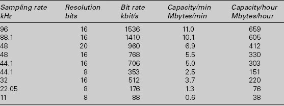
Data rates and capacities for linear PCM
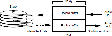
Figure 9.12 RAM buffering is used to convert burst data flow to continuous data flow, and vice versa
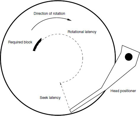
Figure 9.13 The delays involved in accessing a block of data stored on a disk
The number of audio channels that can be recorded or replayed simultaneously depends on the performance of the storage device and the host computer. Slow systems may only be capable of handling a few channels whereas faster systems with multiple disk drives may be capable of expansion up to a virtually unlimited number of channels. Manufacturers are tending to make their systems modular, allowing for expansion of storage and other audio processing facilities as means allow, with all modules communicating over a high-speed data bus, as shown in Figure 9.14. Increasingly disks can be connected using high speed serial interfaces such as Firewire (IEEE 1394), which are fast enough to rival SCSI in some cases (see Fact File 9.6).
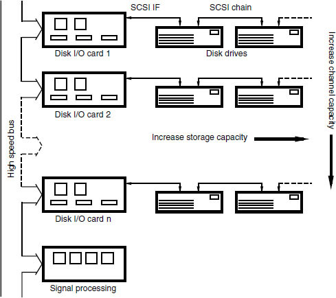
Figure 9.14 Arrangement of multipe disks in a typical modular system, showing how a number of disks can be attached to a single SCSI chain to increase storage capacity. Additional IO cards can be added to increase data throughput for additional audio channels
Disk formatting
The process of formatting a disk or tape erases all of the information in the volume. (It may not actually do this, but it rewrites the directory and volume map information to make it seem as if the disk is empty again.) Effectively the volume then becomes virgin territory again and data can be written anywhere.
When a disk is formatted at a low level the sector headers are written and the bad blocks mapped out. A map is kept of the locations of bad blocks so that they may be avoided in subsequent storage operations. Low-level formatting can take quite a long time as every block has to be addressed. During a high-level format the disk may be subdivided into a number of ‘partitions’. Each of these partitions can behave as an entirely independent ‘volume’ of information, as if it were a separate disk drive (see Figure 9.15). It may even be possible to format each partition in a different way, such that a different filing system may be used for each partition. Each volume then has a directory created, which is an area of storage set aside to contain information about the contents of the disk. The directory indicates the locations of the files, their sizes, and various other vital statistics.
The most common general purpose filing systems in audio workstations are HFS (Hierarchical Filing System) or HFS+ (for Mac OS), FAT 32 (for Windows PCs) and NTFS (for Windows NT and 2000). The Unix operating system is used on some multi-user systems and high-powered workstations and also has its own filing system. These were not designed principally with real-time requirements such as audio and video replay in mind but they have the advantage that disks formatted for a widely used filing system will be more easily interchangeable than those using proprietary systems.
Fact file 9.6 Peripheral interfaces
A variety of different physical interfaces can be used for interconnecting storage devices and host workstations. Some are internal buses only designed to operate over limited lengths of cable and some are external interfaces that can be connected over several metres. The interfaces can be broadly divided into serial and parallel types, the serial types tending to be used for external connections owing to their size and ease of use. The disk interface can be slower than the drive attached to it in some cases, making it into a bottleneck in some applications. There is no point having a super-fast disk drive if the interface cannot handle data at that rate.
SCSI
For many years the most commonly used interface for connecting mass storage media to host computers was SCSI (the Small Computer Systems Interface), pronounced ‘scuzzy’. It is still used quite widely for very high performance applications but EIDE interfaces and drives are now capable of very good performance that can be adequate for many purposes. SCSI is a high-speed parallel interface found on many computer systems, originally allowing up to seven peripheral devices to be connected to a host on a single bus. SCSI has grown through a number of improvements and revisions, the latest being Ultra160 SCSI, capable of addressing 16 devices at a maximum data rate of 160 Mbyte/sec.
ATA/IDE
The ATA and IDE family of interfaces has evolved through the years as the primary internal interface for connecting disk drives to PC system buses. It is cheap and ubiquitous. Although drives with such interfaces were not considered adequate for audio purposes in the past, many people are now using them with the on-board audio processing of modern computers as they are cheap and the performance is adequate for many needs. Recent flavours of this interface family include Ultra ATA/66 and Ultra ATA/100 that use a 40-pin, 80 conductor connector and deliver data rates up to either 66 or 100 Mbyte/sec. ATAPI (ATA Packet Interface) is a variant used for storage media such as CD drives.
Serial ATA is a relatively recent development designed to enable disk drives to be interfaced serially, thereby reducing the physical complexity of the interface. High data transfer rates are planned, eventually up to 600 Mbyte/sec. It is intended primarily for internal connection of disks within host workstations, rather than as an external interface like USB or Firewire.
PCMCIA
PCMCIA is a standard expansion port for notebook computers and other small-size computer products. A number of storage media and other peripherals are available in PCMCIA format, and these include flash memory cards, modem interfaces and super-small hard disk drives. The standard is of greatest use in portable and mobile applications where limited space is available for peripheral storage.
Firewire and USB
Firewire and USB are both serial interfaces for connecting external peripherals. They both enable disk drives to be connected in a very simple manner, with high transfer rates (many hundreds of megabits per second), although USB 1.0 devices are limited to 12 Mbit/s. A key feature of these interfaces is that they can be ‘hot plugged’ (in other words devices can be connected and disconnected with the power on). The interfaces also supply basic power that enables some simple devices to be powered from the host device. Interconnection cables can usually be run up to between 5 and 10 metres, depending on the cable and the data rate, although longer distances may be possible in some cases.
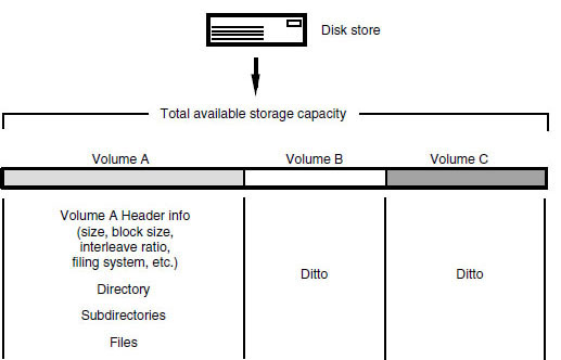
Figure 9.15 A disk may be divided up into a number of different partitions, each acting as an independent volume of information
When an erasable volume like a hard disk has been used for some time there will be a lot of files on the disk, and probably a lot of small spaces where old files have been erased. New files must be stored in the available space and this may involve splitting them up over the remaining smaller areas. This is known as disk fragmentation, and it seriously affects the overall performance of the drive. The reason is clear to see from Figure 9.16. More head seeks are required to access the blocks of a file than if they had been stored contiguously, and this slows down the average transfer rate considerably. It may come to a point where the drive is unable to supply data fast enough for the purpose.
There are only two solutions to this problem: one is to reformat the disk completely (which may be difficult, if one is in the middle of a project), the other is to optimise or consolidate the storage space. Various software utilities exist for this purpose, whose job is to consolidate all the little areas of free space into fewer larger areas. They do this by juggling the blocks of files between disk areas and temporary RAM – a process that often takes a number of hours. Power failure during such an optimisation process can result in total corruption of the drive, because the job is not completed and files may be only half moved, so it is advisable to back up the drive before doing this. It has been known for some such utilities to make the files unusable by some audio editing packages, because the software may have relied on certain files being in certain physical places, so it is wise to check first with the manufacturer.
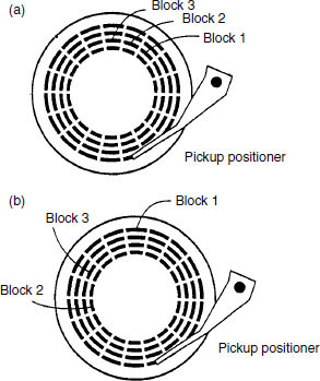
Figure 9.16 At (a) a file is stored in three contiguous blocks and these can be read sequentially without moving the head. At (b) the file is fragmented and is distributed over three remote blocks, involving movement of the head to read it. The latter read operation will take more time
Sound file formats
As the use of networked workstations grows, the need for files to be transferred between systems also grows and either by international standardisation or by sheer force of market dominance certain file formats are becoming the accepted means by which data are exchanged. The recent growth in the importance of metadata (data about data, or strictly ‘beyond data’), and the representation of audio, video and metadata as ‘objects’, has led to the development of interchange methods that are based on object-oriented concepts and project ‘packages’ as opposed to using simple text files and separate media files. There is increasing integration between audio and other media in multimedia authoring and some of the file formats mentioned below are closely related to international efforts in multimedia file exchange. The following is a summary of the most commonly encountered file formats.
Sound Designer formats
Sound Designer files originate with the Californian company Digidesign, manufacturer of probably the world’s most widely used digital audio hardware for desktop computers. Many systems handle Sound Designer files because they were used widely for such purposes as the distribution of sound effects on CD-ROM and for other short music sample files.
The Sound Designer I format (SD I) is for mono sounds and it is recommended principally for use in storing short sounds. It originated on the Macintosh, so numerical data are stored in big-endian byte order but it has no resource fork. The data fork contains a header of 1336 bytes, followed by the audio data bytes. The header contains information about how the sample should be displayed in Sound Designer editing software, including data describing vertical and horizontal scaling. It also contains details of ‘loop points’ for the file (these are principally for use with audio/MIDI sampling packages where portions of the sound are repeatedly cycled through while a key is held down, in order to sustain a note). The header contains information on the sample rate, sample period, number of bits per sample, quantisation method (e.g.: ‘linear’, expressed as an ASCII string describing the method) and size of RAM buffer to be used. The audio data are normally either 8 or 16 bit, and always MSbyte followed by LSbyte of each sample.
Sound Designer II has been one of the most commonly used formats for audio workstations and has greater flexibility than SD I. Again it originated as a Mac file and unlike SD I it has a separate resource fork which contains the file’s ‘vital statistics’. The data fork contains only the audio data bytes in two’s complement form, either 8 or 16 bits per sample. SD II files can contain audio samples for more than one channel, in which case the samples are interleaved, as shown in Figure 9.17, on a sample by sample basis (i.e.: all the bytes for one channel sample followed by all the bytes for the next, etc.). It is unusual to find more than stereo data contained in SD II files and it is recommended that multichannel recordings are made using separate files for each channel.
AIFF and AIFF-C formats
The AIFF format is widely used as an audio interchange standard, because it conforms to the EA IFF 85 standard for interchange format files used for various other types of information such as graphical images. AIFF is an Apple standard format for audio data and is encountered widely on Macintosh-based audio workstations and some Silicon Graphics systems. Audio information can be stored at a number of resolutions and for any number of channels if required, and the related AIFF-C (file type ‘AIFC’) format allows also for compressed audio data. It consists only of a data fork, with no resource fork, making it easier to transport to other platforms.
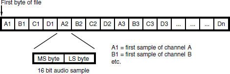
Figure 9.17 Sound Designer II files allow samples for multiple audio channels to be interleaved. Four channel, 16 bit example shown
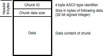
Figure 9.18 General format of an IFF file chunk
All IFF-type files are made up of ‘chunks’ of data which are typically made up as shown in Figure 9.18. A chunk consists of a header and a number of data bytes to follow. The simplest AIFF files contain a ‘common chunk’, which is equivalent to the header data in other audio files, and a ‘sound data’ chunk containing the audio sample data. These are contained overall by a ‘form’ chunk as shown in Figure 9.19. AIFC files must also contain a ‘Version Chunk’ before the common chunk to allow for future changes to AIFC.
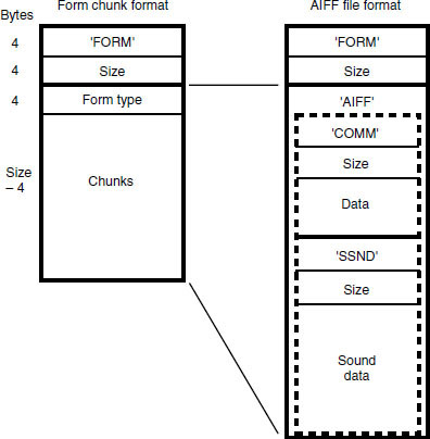
Figure 9.19 General format of an AIFF file
RIFF WAVE format
The RIFF WAVE (often called WAV) format is the Microsoft equivalent of Apple’s AIFF. It has a similar structure, again conforming to the IFF pattern, but with numbers stored in little-endian rather than big-endian form. It is used widely for sound file storage and interchange on PC workstations, and for multimedia applications involving sound. Within WAVE files it is possible to include information about a number of cue points, and a playlist to indicate the order in which the cues are to be replayed. WAVE files use the file extension ‘.wav’.
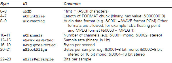
A basic WAV file consists of three principal chunks, as shown in Figure 9.20, the RIFF chunk, the FORMAT chunk and the DATA chunk. The RIFF chunk contains 12 bytes, the first four of which are the ASCII characters ‘RIFF’, the next four indicating the number of bytes in the remainder of the file (after the first eight) and the last four of which are the ASCII characters ‘WAVE’. The format chunk contains information about the format of the sound file, including the number of audio channels, sampling rate and bits per sample, as shown in Table 9.1.
The audio data chunk contains a sequence of bytes of audio sample data, divided as shown in the FORMAT chunk. Unusually, if there are only eight bits per sample or fewer each value is unsigned and ranges between 0 and 255 (decimal), whereas if the resolution is higher than this the data are signed and range both positively and negatively around zero. Audio samples are interleaved by channel in time order, so that if the file contains two channels a sample for the left channel is followed immediately by the associated sample for the right channel. The same is true of multiple channels (one sample for time-coincident sample periods on each channel is inserted at a time, starting with the lowest numbered channel), although basic WAV files were nearly always just mono or two channel.
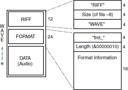
Figure 9.20 Diagrammatic representation of a simple RIFF WAVE file, showing the three principal chunks. Additional chunks may be contained within the overall structure, for example a ‘bext’ chunk for the Broadcast WAVE file
Table 9.1 Contents of FORMAT chunk in a basic WAVE PCM file
The RIFF WAVE format is extensible and can have additional chunks to define enhanced functionality such as surround sound and other forms of coding. This is known as ‘WAVE-format extensible’ (see http://www.microsoft.com/hwdev/tech/audio/multichaud.asp). Chunks can include data relating to cue points, labels and associated data, for example. The Broadcast WAVE format is one example of an enhanced WAVE file (see Fact File 9.7).
MPEG audio file formats
It is possible to store MPEG-compressed audio in AIFF-C or WAVE files, with the compression type noted in the appropriate header field. There are also older MS-DOS file extensions used to denote MPEG audio files, notably .MPA (MPEG Audio) or .ABS (Audio Bit Stream). However, owing to the ubiquity of the so-called ‘MP3’ format (MPEG 1, Layer 3) for audio distribution on the Internet, MPEG audio files are increasingly denoted with the extension ‘.MP3’. Such files are relatively simple, being really no more than MPEG audio frame data in sequence, each frame being preceded by a frame header.
DSD-IFF file format
The DSD-IFF file format is based on a similar structure to other IFF-type files, described above, except that it is modified slightly to allow for the large file sizes that may be encountered with the high resolution Direct Stream Digital format used for SuperAudio CD. Specifically the container FORM chunk is labelled ‘FRM8’ and this identifies all local chunks that follow as having ‘length’ indications that are eight bytes long rather than the normal four. In other words, rather than a four-byte chunk ID followed by a four-byte length indication, these files have a four-byte ID followed by an eight-byte length indication. This allows for the definition of chunks with a length greater than 2 Gbytes, which may be needed for mastering SuperAudio CDs. There are also various optional chunks that can be used for exchanging more detailed information and comments such as might be used in project interchange. Further details of this file format, and an excellent guide to the use of DSD-IFF in project applications, can be found in the DSD-IFF specification, as described in the Recommended further reading at the end of this chapter.
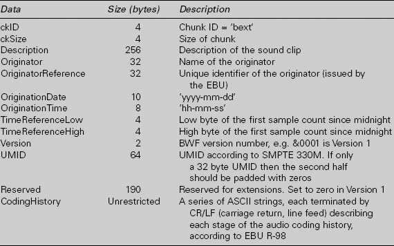
Fact file 9.7 Broadcast WAVE format
The Broadcast WAVE format, described in EBU Tech. 3285, was standardised by the European Broadcasting Union (EBU) because of a need to ensure compatibility of sound files and accompanying information when transferred between workstations. It is based on the RIFF WAVE format described above, but contains an additional chunk that is specific to the format (the ‘broadcast_audio_extension’ chunk, ID = ‘bext’) and also limits some aspects of the WAVE format. Version 0 was published in 1997 and Version 1 in 2001, the only difference being the addition of an SMPTE UMID (Unique Material Identifier) in version 1 (this is a form of metadata). Such files currently only contain either PCM or MPEG-format audio data.
Broadcast WAVE files contain at least three chunks: the broadcast_audio_extension chunk, the format chunk and the audio data chunk. The broadcast extension chunk contains the data shown in the table below. Optionally files may also contain further chunks for specialised purposes and may contain chunks relating to MPEG audio data (the ‘fact’ and ‘mpeg_audio_ extension’ chunks). MPEG applications of the format are described in EBU Tech. 3285, Supplement 1 and the audio data chunk containing the MPEG data normally conforms to the MP3 frame format.
A multichannel extension chunk has recently been proposed for Broadcast WAVE files that define the channel ordering, surround format, downmix coefficients for creating a two-channel mix, and some descriptive information. There are also chunks defined for metadata describing the audio contained within the file, such as the ‘quality chunk’ (ckID = ‘qlty’), which together with the coding history contained in the ‘bext’ chunk make up the so-called ‘capturing report’. These are described in Supplement 2 to EBU Tech. 3285. Finally there is a chunk describing the peak audio level within a file, which can aid automatic programme level setting and programme interchange.
Broadcast audio extension chunk format
Edit decision list (EDL) files
EDL formats have usually been unique to the workstation on which they are used but the need for open interchange is increasing the pressure to make EDLs transportable between packages. There is an old and widely used format for EDLs in the video world that is known as the CMX-compatible form. CMX is a well-known manufacturer of video editing equipment and most editing systems will read CMX EDLs for the sake of compatibility. These can be used for basic audio purposes, and indeed a number of workstations can read CMX EDL files for the purpose of auto-conforming audio edits to video edits performed on a separate system. The CMX list defines the cut points between source material and the various transition effects at joins, and it can be translated reasonably well for the purpose of defining audio cut points and their timecode locations, using SMPTE/EBU form, provided video frame accuracy is adequate.
Software can be obtained for audio and video workstations that translates EDLs between a number of different standards to make interchange easier, although it is clear that this process is not always problem-free and good planning of in-house processes is vital. The OMFI (Open Media Framework Interchange) structure also contains a format for interchanging edit list data. AES-31 is now gaining considerable popularity among workstation software manufacturers as a simple means of exchanging audio editing projects between systems. The Advanced Authoring Format (AAF) is becoming increasingly relevant to the exchange of media project data between systems, and is likely to take over from OMFI as time progresses.
MXF – the Media Exchange Format
MXF was developed by the Pro-MPEG forum as a means of exchanging audio, video and metadata between devices, primarily in television operations. It is based on the modern concept of media objects that are split into ‘essence’ and ‘metadata’. Essence files are the raw material (i.e.: audio and video) and the metadata describes things about the essence (such as where to put it, where it came from and how to process it).
MXF files attempt to present the material in a ‘streaming’ format, that is one that can be played out in real time, but they can also be exchanged in conventional file transfer operations. As such they are normally considered to be finished programme material, rather than material that is to be processed somewhere downstream, designed for playout in broadcasting environments. The bit stream is also said to be compatible with recording on digital videotape devices.
AAF – the Advanced Authoring Format
AAF is an authoring format for multimedia data that is supported by numerous vendors, including Avid which has adopted it as a migration path from OMFI. Parts of OMFI 2.0 form the basis for parts of AAF and there are also close similarities between AAF and MXF (described in the previous section). Like the formats to which it has similarities, AAF is an object-oriented format that combines essence and metadata within a container structure. Unlike MXF it is designed for project interchange such that elements within the project can be modified, post-processed and resynchronised. It is not, therefore, directly suitable as a streaming format but can easily be converted to MXF for streaming if necessary.
Rather like OMFI it is designed to enable complex relationships to be described between content elements, to map these elements onto a timeline, to describe the processing of effects, synchronise streams of essence, retain historical metadata and refer to external essence (essence not contained within the AAF package itself). It has three essential parts: the AAF Object Specification (which defines a container for essence and metadata, the logical contents of objects and rules for relationships between them); the AAF Low-Level Container Specification (which defines a disk filing structure for the data, based on Microsoft’s Structured Storage); and the AAF SDK Reference Implementation (which is a software development kit that enables applications to deal with AAF files). The Object Specification is extensible in that it allows new object classes to be defined for future development purposes.
Consumer digital formats
Compact Discs and drives
The CD is not immediately suitable for real-time audio editing and production, partly because of its relatively slow access time compared with hard disks, but can be seen to have considerable value for the storage and transfer of sound material that does not require real-time editing. Broadcasters use them for sound effects libraries and studios and mastering facilities use them for providing customers and record companies with ‘acetates’ or test pressings of a new recording. They have also become quite popular as a means of transferring finished masters to a CD pressing plant in the form of the PMCD (pre-master CD). They are ideal as a means of ‘proofing’ CD-ROMs and other CD formats, and can be used as low cost backup storage for computer data.
Compact Discs (CDs) are familiar to most people as a consumer read-only optical disc for audio (CD-DA) or data (CD-ROM) storage. Standard audio CDs (CD-DA) conform to the Red Book standard published by Philips. The CD-ROM standard (Yellow Book) divides the CD into a structure with 2048 byte sectors, adds an extra layer of error protection, and makes it useful for general purpose data storage including the distribution of sound and video in the form of computer data files. It is possible to find discs with mixed modes, containing sections in CD-ROM format and sections in CD-Audio format. The CD Plus is one such example.
CD-R is the recordable CD, and may be used for recording CD-Audio format or other CD formats using a suitable drive and software. The Orange Book, Part 2, contains information on the additional features of CD-R, such as the area in the centre of the disc where data specific to CD-R recordings is stored. Audio CDs recorded to the Orange Book standard can be ‘fixed’ to give them a standard Red Book table of contents (TOC), allowing them to be replayed on any conventional CD player. Once fixed into this form, the CD-R may not subsequently be added to or changed, but prior to this there is a certain amount of flexibility, as discussed below. CD-RW discs are erasable and work on phase-change principles, requiring a drive compatible with this technology, being described in the Orange Book, Part 3.
The degree of reflectivity of CD-RW discs is much lower than that of typical CD-R and CD-ROM. This means that some early drives and players may have difficulties reading them. However, the ‘multi-read’ specification developed by the OSTA (Optical Storage Technology Association) describes a drive that should read all types of CD, so recent drives should have no difficulties here.
MiniDisc
CD has been available for some years now as a 16 bit 44.1 kHz digital playback medium; it was joined by CD-ROM, CD-R (recordable) and CD-RW (recordable and rewritable). The MiniDisc (MD) is now an established consumer recording and playback format, and it is of the M-O (magneto-optical) type. Sampling frequency is fixed at 44.1 kHz, and resolution is nominally 16 bit. A coding system similar to those originally developed for digital audio broadcasting (DAB) known as Adaptive Transform Acoustic Coding (ATRAC) is used whereby the incoming signal is first split into three bands: below 5.5 kHz, 5.5–11 kHz, and above 11 kHz, and each band is individually analysed with respect to frequency content and level over successive short periods of time via Modified Discrete Cosine Transform (MDCT) filter blocks. Within the three blocks, non-uniform frequency splitting into 20, 16 and 16 further sub-bands takes place, and the circuit then discards material which it deems will be masked by other sounds which are present at higher signal levels and/or have a similar frequency content. A data rate of about one fifth that required for CD is adequate to encode the resulting signal (CD’s data stream is 1.4 Mb/s, MD’s is 292 Kb/s) and this allows usefully long playing times to be obtained from a disc which is somewhat smaller than a CD at 64 mm in diameter. Since the format involves considerable data compression (a slight misnomer for data reduction), it is not suitable for professional master recording or archiving, but is used quite widely in applications where the highest sound quality is not required such as broadcast journalism.
DVD
DVD is the natural successor to CD, being a higher density optical disc format aimed at the consumer market, having the same diameter as CD and many similar physical features. It uses a different laser wavelength to CD (635–650 nm as opposed to 780 nm) so multi-standard drives need to be able to accommodate both. Data storage capacity depends on the number of sides and layers to the disc, but ranges from 4.7 Gbytes (single-layer, single-sided) up to about 18 Gbytes (double-layer, double-sided). The data transfer rate at ‘one times’ speed is just over 11 Mbit/s.
DVD can be used as a general purpose data storage medium. Like CD, there are numerous different variants on the recordable DVD, partly owing to competition between the numerous different ‘factions’ in the DVD consortium. These include DVD-R, DVD-RAM, DVD-RW and DVD+RW, all of which are based on similar principles but have slightly different features, leading to a compatibility minefield that is only gradually being addressed (see Fact File 9.8). The ‘DVD Multi’guidelines produced by the DVD Forum are an attempt to foster greater compatibility between DVD drives and discs, but this does not really solve the problem of the formats that are currently outside the DVD Forum.
Fact file 9.8 Recordable DVD formats
Recordable DVD type | Description |
DVD-R (A and G) | DVD equivalent of CD-R. One-time recordable in sequential manner, replayable on virtually any DVD-ROM drive. Supports ‘incremental writing’ or ‘disc at once’ recording. Capacity either 3.95 (early discs) or 4.7 Gbyte per side. ‘Authoring’ (A) version (recording laser wavelength = 635 nm) can be used for pre-mastering DVDs for pressing, including DDP data for disc mastering (see Chapter 6). ‘General’ (G) version (recording laser wavelength = 650 nm) intended for consumer use, having various ‘content protection’ features that prevent encrypted commercial releases from being cloned |
DVD-RAM | Sectored format, rather more like a hard disk in data structure when compared with DVD-R. Uses phase-change (PD-type) principles allowing direct overwrite. Version 2 discs allow 4.7 Gbyte per side (reduced to about 4.2 Gbyte after formatting). Type 1 cartridges are sealed and Type 2 allow the disc to be removed. Double-sided discs only come in sealed cartridges. Can be rewritten about 100 000 times. The recent Type 3 is a bare disc that can be placed in an open cartridge for recording |
DVD-RW | Pioneer development, similar to CD-RW in structure, involving sequential writing. Does not involve a cartridge. Can be rewritten about 1000 times. 4.7 Gbyte per side |
DVD+RW | Non-DVD-Forum alternative to DVD-RAM (and not compatible), allowing direct overwrite. No cartridge. Data can be written in either CLV (for video recording) or CAV (for random access storage) modes. There is also a write-once version known as DVD+R |
Writeable DVDs are a useful option for backup of large projects, particularly DVD-RAM because of its many-times overwriting capacity and its hard disk-like behaviour. It is possible that a format like DVD-RAM could be used as primary storage in a multitrack recording/editing system, as it has sufficient performance for a limited number of channels and it has the great advantage of being removable. However, it is likely that hard disks will retain the performance edge for the foreseeable future.
DVD-Video is the format originally defined for consumer distribution of movies with surround sound, typically incorporating MPEG-2 video encoding and Dolby Digital surround sound encoding. It also allows for up to eight channels of 48 or 96 kHz linear PCM audio, at up to 24 bit resolution. DVD-Audio is intended for very high quality multichannel audio reproduction and allows for linear PCM sampling rates up to 192 kHz, with numerous configurations of audio channels for different surround modes, and optional lossless data reduction (MLP).
DVD-Audio has a number of options for choosing the sampling frequencies and resolutions of different channel groups, it being possible to use a different resolution on the front channels from that used on the rear, for example. The format is more versatile in respect of sampling frequency than DVD-Video, having also accommodated multiples of the CD sample frequency of 44.1 kHz as options (the DVD-Video format allows only for multiples of 48 kHz). Consequently, the allowed sample frequencies for DVD-Audio are 44.1, 48, 88.2, 96, 176.4, 192 kHz. The sample frequencies are split into two groups – multiples of 44.1 and multiples of 48 kHz. While it is possible to split frequencies from one group among the audio channels on a DVD-A (see below), one cannot combine frequencies across the groups for reasons of simple clock rate division. Bit resolution can be 16, 20 or 24 bits per channel, and again this can be divided unequally between the channels, according to the channel group split described below.
Meridian Lossless Packing (MLP) is licensed through Dolby Laboratories and is a lossless coding technique designed to reduce the data rate of audio signals without compromising sound quality. It has both a variable bit rate mode and a fixed bit rate mode. The variable mode delivers the optimum compression for storing audio in computer data files, but the fixed mode is important for DVD applications where one must be able to guarantee a certain reduction in peak bit rate.
Super Audio CD (SACD)
Version 1.0 of the SACD specification is described in the ‘Scarlet Book’, available from Philips licensing department. SACD uses DSD (Direct Stream Digital) as a means of representing audio signals, as described in Chapter 2, so requires audio to be sourced in or converted to this form. SACD aims to provide a playing time of at least 74 minutes for both two channel and six channel balances. The disc is divided into two regions, one for two-channel audio, the other for multichannel, as shown in Figure 9.21. A lossless data packing method known as Direct Stream Transfer (DST) can be used to achieve roughly 2:1 data reduction of the signal stored on disc so as to enable high quality multichannel audio on the same disc as the two channel mix.
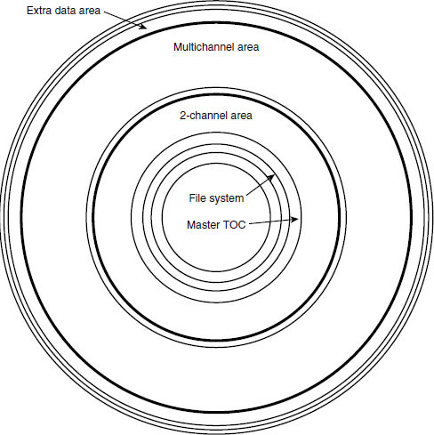
Figure 9.21 Different regions of a Super Audio CD, showing separate two-channel and multichannel regions
SACDs can be manufactured as single or dual-layer discs, with the option of the second layer being a Red Book CD layer (the so-called ‘hybrid disc’). SACDs, not being a formal part of the DVD hierarchy of standards (although using some of the optical disc technology), do not have the same options for DVD-Video objects as DVD-Audio. The disc is designed first and foremost as a super-high quality audio medium. Nonetheless there is provision for additional data in a separate area of the disc. The content and capacity of this is not specified but could be video clips, text or graphics, for example.
Solid state recording formats
The capacity and cheapness of solid state RAM (random access memory) makes it increasingly suitable as a storage format for digital audio. In consumer form this is evident in the proliferation of ‘memory stick’ MP3 players, for example. In the professional environment solid state memory recorders are sometimes used in broadcasting applications, for portable use by journalists, for example. Recordings are usually made in a data-reduced format in order to make optimum use of limited memory, and a variety of interfaces such as telephone, ISDN and Ethernet may be available for transferring the stored audio to more permanent storage at a broadcasting centre.
Audio processing for computer workstations
Introduction
A lot of audio processing now takes place within the workstation, usually relying either on the host computer’s processing power (using the CPU to perform signal processing operations) or on one or more DSP (digital signal processing) cards attached to the workstation’s expansion bus. Professional systems usually use external A/D and D/A convertors, connected to a ‘core’ card attached to the computer’s expansion bus. This is because it is often difficult to obtain the highest technical performance from convertors mounted on internal sound cards, owing to the relatively ‘noisy’ electrical environment inside most computers. Furthermore, the number of channels required may not fit onto an internal card. As more and more audio work takes place entirely in the digital domain, though, the need for analogue convertors decreases. Digital interfaces are also often provided on external ‘breakout boxes’, partly for convenience and partly because of physical size of the connectors. Compact connectors such as the optical connector used for the ADAT eight-channel interface or the two-channel SPDIF phono connector are accommodated on some cards, but multiple AES/EBU connectors cannot be.
It is also becoming increasingly common for substantial audio processing power to exist on integrated sound cards that contain digital interfaces and possibly A/D and D/A convertors. These cards are typically used for consumer or semi-professional applications on desktop computers, although many now have very impressive features and can be used for advanced operations. Such cards are now available in ‘full duplex’ configurations that enable audio to be received by the card from the outside world, processed and/or stored, then routed back to an external device. Full duplex operation usually allows recording and replay simultaneously.
Sound cards and DSP cards are commonly connected to the workstation using the PCI (peripheral component interface) expansion bus. Older ISA (PC) buses or NuBus (Mac) slots did not have the same data throughput capabilities and performance was therefore somewhat limited. PCI can be extended to an external expansion chassis that enables a larger number of cards to be connected than allowed for within the host computer. Sufficient processing power can now be installed for the workstation to become the audio processing ‘heart’ of a larger studio system, as opposed to using an external mixing console and effects units. The higher the sampling frequency, the more DSP operations will be required per second, so it is worth bearing in mind that going up to, say, 96 kHz sampling frequency for a project will require double the processing power and twice the storage space of 48 kHz. The same is true of increasing the number of channels to which processing is applied.
Fact file 9.9 Audio processing latency
Latency is the delay incurred in executing audio operations between input and output of a system. The lower the better is the rule, particularly when operating systems in ‘full duplex’ mode, because processed sound may be routed back to musicians (for foldback purposes) or may be combined with undelayed sound at some point. The management of latency is a software issue and some systems have sophisticated approaches to ensuring that all supposedly synchronous audio reaches the output at the same time no matter what processing it has encountered on the way.
Minimum latency achievable is both a hardware and a software issue. The poorest systems can give rise to tens or even hundreds of milliseconds between input and output whereas the best reduce this to a few milliseconds. Audio I/O that connects directly to an audio processing card can help to reduce latency, otherwise the communication required between host and various cards can add to the delay. Some real-time audio processing software also implements special routines to minimise and manage critical delays and this is often what distinguishes professional systems from cheaper ones. The audio driver software or ‘middleware’ that communicates between applications and sound cards influences latency considerably. One example of such middleware intended for low latency audio signal routing in computers is Steinberg’s ASIO (Audio Stream Input Output).
The issue of latency is important in the choice of digital audio hardware and software, as discussed in Fact File 9.9.
DSP cards
DSP cards can be added to widely used workstation packages such as Digidesign’s ProTools. These so-called ‘DSP Farms’ or ‘Mix Farms’ are expansion cards that connect to the PCI bus of the workstation and take on much of the ‘number crunching’ work involved in effects processing and mixing. ‘Plug-in’ processing software is becoming an extremely popular and cost-effective way of implementing effects processing within the workstation, and this is discussed further in Chapter 10. ProTools plug-ins usually rely either on DSP Farms or on host-based processing (see the next section) to handle this load.
Digidesign’s TDM (Time Division Multiplex) architecture is a useful example of the way in which audio processing can be handled within the workstation. Here the processing tasks are shared between DSP cards, each card being able to handle a certain number of operations per second. If the user runs out of ‘horse power’ it is possible to add further DSP cards to share the load. Audio is routed and mixed at 24 bit resolution, and a common audio bus links the card that is connected on a separate multiway ribbon cable.
Host-based audio processing
An alternative to using dedicated DSP cards is to use the now substantial processing capacity of a typical desktop workstation. The success of such ‘host-based processing’ obviously depends on the number of tasks that the workstation is required to undertake and this capacity may vary with time and context. It is, however, quite possible to use the host’s own CPU to run DSP ‘plug-ins’ for implementing equalisation, mixing and limited effects, provided it is fast enough.
The software architecture required to run plug-in operations on the host CPU is naturally slightly different to that used on dedicated DSP cards, so it is usually necessary to specify whether the plug-in is to run on the host or on a dedicated resource such as Digidesign’s TDM cards. A number of applications are now appearing, however, that enable the integration of host-based (or ‘native’) plug-ins and dedicated DSP such as TDM-bus cards. Audio processing that runs on the host may be subject to greater latency (input to output delay) than when using dedicated signal processing, and it obviously takes up processing power that could be used for running the user interface or other software. It is nonetheless a cost-effective option for many users that do not have high expectations of a system and it may be possible to expand the system to include dedicated DSP in the future.
Integrated sound cards
Integrated sound cards typically contain all the components necessary to handle audio for basic purposes within a desktop computer and may be able to operate in full duplex mode (in and out at the same time). They typically incorporate convertors, DSP, a digital interface, FM and/or wavetable synthesis engines. Optionally, they may also include some sort of I/O daughter board that can be connected to a break-out audio interface, increasing the number of possible connectors and the options for external analogue conversion. Such cards also tend to sport MIDI/joystick interfaces. A typical example of this type of card is the ‘SoundBlaster’ series from Creative Labs.
Any analogue audio connections are normally unbalanced and the convertors may be of only limited quality compared with the best external devices. For professional purposes it is advisable to use high quality external convertors and balanced analogue audio connections.
Disk-based editing system principles
Introduction
The random access nature of disk-based mass storage media led to the coining of the term non-linear editing for the process of audio editing. With non-linear editing the editor may preview a number of possible masters in their entirety before deciding which should be the final one. Even after this, it is a simple matter to modify the edit list to update the master. Edits may also be previewed and experimented with in order to determine the most appropriate location and processing. Crossfades may be modified and adjustments made to equalisation and levels, all in the digital domain. Non-linear editing has also come to feature very widely in post-production for video and film.
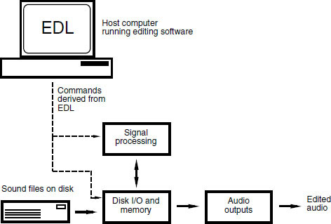
Figure 9.22 Instructions from an edit decision list (EDL) are used to control the replay of sound file segments from disk, which may be subjected to further processing (also under EDL control) before arriving at the audio outputs
Non-linear editing is truly non-destructive in that the edited master only exists as a series of instructions to replay certain parts of sound files at certain times, with specified signal processing overlaid, as shown in Figure 9.22. The original sound files remain intact at all times, and a single sound file can be used as many times as desired in different locations and on different tracks without the need for copying the audio data. Editing may involve the simple joining of sections, or it may involve more complex operations such as long crossfades between one album track and the next, or gain offsets between one section and another. All these things are possible without affecting the original source material.
Sound files and sound segments
In the case of music editing sound files might be session takes, anything from a few bars to a whole movement, while in picture dubbing they might contain a phrase of dialogue or a sound effect. Specific segments of these sound files can be defined while editing, in order to get rid of unwanted material or to select useful extracts. The terminology varies but such identified parts of sound files are usually termed either ‘clips’ or ‘segments’. Rather than creating a copy of the segment or clip and storing it as a separate sound file, it is normal simply to store it as a ‘soft’ entity – in other words as simply commands in an edit list or project file that identify the start and end addresses of the segment concerned and the sound file to which it relates. It may be given a name by the operator and subsequently used as if it were a sound file in its own right. An almost unlimited number of these segments can be created from original sound files, without the need for any additional audio storage space.
Edit point handling
Edit points can be simple butt joins or crossfades. A butt join is very simple because it involves straightforward switching from the replay of one sound segment to another. Since replay involves temporary storage of the sound file blocks in RAM (see above) it is a relatively simple matter to ensure that both outgoing and incoming files in the region of the edit are available in RAM simultaneously (in different address areas). Up until the edit, blocks of the outgoing file are read from the disk into RAM and thence to the audio outputs. As the edit point is reached a switch occurs between outgoing and incoming material by instituting a jump in the memory read address corresponding to the start of the incoming material. Replay then continues by reading subsequent blocks from the incoming sound file. It is normally possible to position edits to single sample accuracy, making the timing resolution as fine as a number of tens of microseconds if required.
The problem with butt joins is that they are quite unsubtle. Audible clicks and bumps may result because of the discontinuity in the waveform that may result, as shown in Figure 9.23. It is normal, therefore, to use at least a short crossfade at edit points to hide the effect of the join. This is what happens when analogue tape is spliced, because the traditional angled cut has the same effect as a short crossfade (of between 5 and 20 ms depending on the tape speed and angle of cut). Most workstations have considerable flexibility with crossfades and are not limited to short durations. It is now common to use crossfades of many shapes and durations (e.g.: linear, root cosine, equal power) for different creative purposes. This, coupled with the ability to preview edits and fine-tune their locations, has made it possible to put edits in places previously considered impossible.
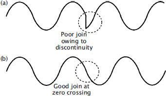
Figure 9.23 (a) A bad butt edit results in a waveform discontinuity. (b) Butt edits can be made to work if there is minimal discontinuity
The locations of edit points are kept in an edit decision list (EDL) which contains information about the segments and files to be replayed at each time, the in and the out points of each section and details of the crossfade time and shape at each edit point. It may also contain additional information such as signal processing operations to be performed (gain changes, EQ, etc.).
Crossfading
Crossfading is similar to butt joining, except that it requires access to data from both incoming and outgoing files for the duration of the crossfade. The crossfade calculation involves simple signal processing, during which the values of outgoing samples are multiplied by gradually decreasing coefficients whilst the values of incoming samples are multiplied by gradually increasing coefficients. Time coincident samples of the two files are then added together to produce output samples, as described in the previous chapter. The duration and shape of the crossfade can be adjusted by altering the coefficients involved and the rate at which the process is executed.
Crossfades are either performed in real time, as the edit point passes, or precalculated and written to disk as a file. Real-time crossfades can be varied at any time and are simply stored as commands in the EDL, indicating the nature of the fade to be executed. The process is similar to that for the butt edit, except that as the edit point approaches samples from both incoming and outgoing segments are loaded into RAM in order that there is an overlap in time. During the crossfade it is necessary to continue to load samples from both incoming and outgoing segments into their respective areas of RAM, and for these to be routed to the crossfade processor, as shown in Figure 9.24. The resulting samples are then available for routing to the output. Alternatively the crossfade can be calculated in non-real time. This incurs a short delay while the system works out the sums, after which a new sound file is stored which contains only the crossfade. Replay of the edit then involves playing the outgoing segment up to the beginning of the crossfade, then the crossfade file, then the incoming segment from after the crossfade, as shown in Figure 9.25. Load on the disk drive is no higher than normal in this case.
The shape of the crossfade can usually be changed to suit different operational purposes. Standard linear fades (those where the gain changes uniformly with time) are not always the most suitable for music editing, especially when the crossfade is longer than about ten millseconds. The result may be a momentary drop in the resulting level in the centre of the crossfade that is due to the way in which the sound levels from the two files add together. If there is a random phase difference between the signals, as there will often be in music, the rise in level resulting from adding the two signals will normally be around 3 dB, but the linear crossfade is 6 dB down in its centre resulting in an overall level drop of around 3 dB (see Figure 9.26). Exponential crossfades and other such shapes may be more suitable for these purposes, because they have a smaller level drop in the centre. It may even be possible to design customised crossfade laws. It is often possible to alter the offset of the start and end of the fade from the actual edit point and to have a faster fade-up than fade-down.
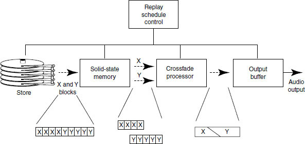
Figure 9.24 Conceptual diagram of the sequence of operations which occur during a crossfade. X and Y are the incoming and outgoing sound segments
Many systems also allow automated gain changes to be introduced as well as fades, so that level differences across edit points may be corrected. Figure 9.27 shows a crossfade profile which has a higher level after the edit point than before it, and different slopes for the in and out fades. A lot of the difficulties that editors encounter in making edits work can be solved using a combination of these facilities.
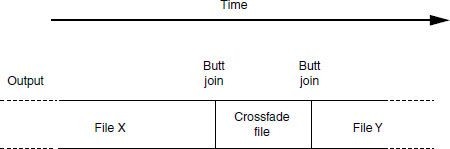
Figure 9.25 Replay of a precalculated crossfade file at an edit point between files X and Y
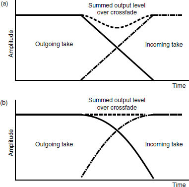
Figure 9.26 Summation of levels at a crossfade. (a) A linear crossfade can result in a level drop if the incoming and outgoing material are non-coherent. (b) An exponential fade, or other similar laws, can help to make the level more constant across the edit
Editing modes
During the editing process the operator will load appropriate sound files and audition them, both on their own and in a sequence with other files. The exact method of assembling the edited sequence depends very much on the user interface, but it is common to present the user with a visual analogy of moving tape, allowing files to be ‘cut and spliced’ or ‘copied and pasted’ into appropriate locations along the virtual tape. These files, or edited clips of them, are then played out at the timecode locations corresponding to their positions on this ‘virtual tape’. It is also quite common to display a representation of the audio waveform that allows the editor to see as well as hear the signal around the edit point (see Figure 9.28).
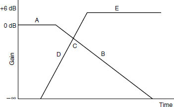
Figure 9.27 The system may allow the user to program a gain profile around an edit point, defining the starting gain (A), the fade-down time (B), the fade-up time (D), the point below unity at which the two files cross over (C) and the final gain (E)
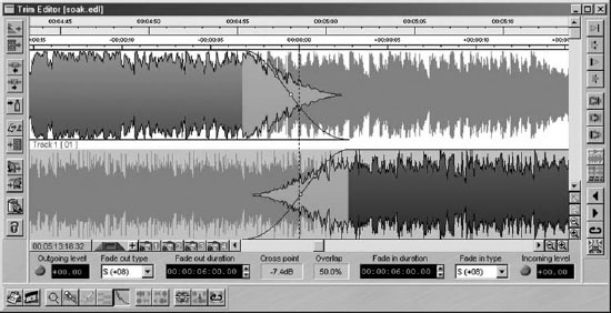
Figure 9.28 Example from SADiE editing system showing the ‘trim editor’ in which is displayed a detailed view of the audio waveform around the edit point, together with information about the crossfade
In non-linear systems the tape-based approach is often simulated, allowing the user to roughly locate an edit point while playing the virtual tape followed by a fine trim using simulated reel-rocking or a detailed view of the waveform. Some software presents source and destination streams as well, in further simulation of the tape approach. It is also possible to insert or change sections in the middle of a finished master, provided that the EDL and source files are still available. To take an example, assume that an edited opera has been completed and that the producer now wishes to change a take somewhere in the middle (see Figure 9.29). The replacement take is unlikely to be exactly the same length but it is possible simply to shuffle all of the following material along or back slightly to accommodate it, this being only a matter of changing the EDL rather than modifying the stored music in any way. The files are then simply played out at slightly different times than in the first version of the edit.
It is also normal to allow edited segments to be fixed in time if desired, so that they are not shuffled forwards or backwards when other segments are inserted. This ‘anchoring’ of segments is often used in picture dubbing when certain sound effects and dialogue have to remain locked to the picture.
Simulation of ‘reel-rocking’
It is common to simulate the effect of analogue tape ‘reel-rocking’ in non-linear editors, providing the user with the sonic impression that reels of analogue tape are being ‘rocked’ back and forth as they are in analogue tape editing when fine-searching edit points. Editors are used to the sound of tape moving in this way, and are skilled at locating edit points when listening to such a sound.
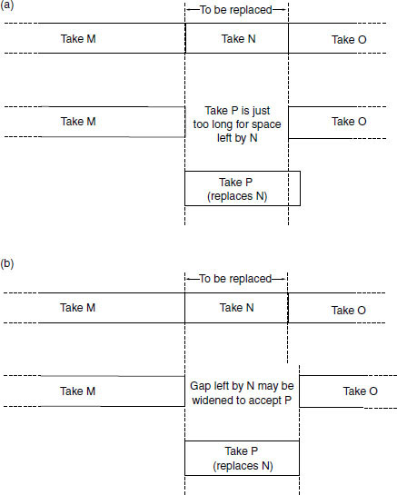
Figure 9.29 Replacing a take in the middle of an edited programme. (a) Tape based copy editing results in a gap of fixed size, which may not match the new take length. (b) Non-linear editing allows the gap size to be adjusted to match the new take
The simulation of variable speed replay in both directions (forwards and backwards) is usually controlled by a wheel or sideways movement of a mouse which moves the ‘tape’ in either direction around the current play location. The magnitude and direction of this movement is used to control the rate at which samples are read from the disk file, via the buffer, and this replaces the fixed sampling rate clock as the controller of the replay rate. Systems differ very greatly as to the sound quality achieved in this mode, because it is in fact quite a difficult task to provide convincing simulation. So poor have been many attempts that many editors do not use the feature, preferring to judge edit points accurately ‘on the fly’, followed by trimming or nudging them either way if they are not successful the first time. Good simulation requires very fast, responsive action and an ergonomically suitable control. A mouse is very unsuitable for the purpose. It also requires a certain amount of DSP to filter the signal correctly, in order to avoid the aliasing that can be caused by varying the sampling rate.
Recommended further reading
Rumsey, F. (2004) Desktop Audio Technology. Focal Press
Watkinson, J. (2001) The Art of Digital Audio. Focal Press