
Introduction to Hypothesis Testing
JMP and Inferences about One Variable
Inferences about Variances and Standard Deviations
Bootstrapping Inference about the Median
Finding the Right Sample Size for Proportions
We now have the tools to introduce the basic logic of inferential statistics. The ideas introduced in this chapter will be used throughout the rest of the text. To set the stage for our discussion, we will first go back to a figure introduced in the last chapter (Figure 6.1).
Figure 6.1 Inductive and Deductive Reasoning in Statistics
In Chapter 5, we discussed the concept of sampling distributions that allowed us to deduce what we were likely to observe for values of sample statistics when samples are taken from a population with known characteristics. We will now use these same sampling distributions to discuss how we can infer something about an unknown population on the basis of a sample with known characteristics. In the last chapter, we discussed ways to find both quantiles for probability distributions and also probabilities from those distributions. In this chapter, we will use the quantiles from the sampling distributions to form interval estimates, and the probabilities will be used in hypothesis testing. In this way, sampling distributions become the bridge that we can use for inferential statistics. It is important to keep in mind that statistical inference is an inductive process as indicated in Figure 6.1. This means that even if we do everything right, our inferences may be wrong. However, the proper use of statistical inference produces rational decisions that have the best chance of being correct.
Inferential statistics is traditionally divided into two areas: estimation and hypothesis testing. Although there is a great deal of overlap between the two, as we shall see later, we will continue this tradition in our discussions here.
The Situation at INCU
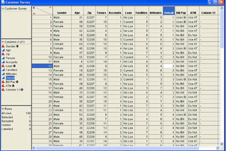
Ann Rigney, the VP of Marketing at INCU, has been looking over some of the data that Betty Anderson gathered during a customer survey she conducted (and which was described in Chapter 4). The data contained information on customer demographics such as gender (male or female), age in years, and zip code of their home address. There is also information on how long the customer has been with INCU in months, how many accounts they have with INCU, and whether or not they have current loans with INCU. The data also contains responses to three questions related to customer satisfaction that were answered on a 7-point scale from 1 (Very Unsatisfied) to 7 (Very Satisfied). The three questions were: satisfaction with the physical facilities at INCU, satisfaction with the attitudes and capabilities of the employees at INCU, and an overall satisfaction with the services of INCU. In addition, there is information on whether the customers use the online bill paying system at INCU and if they used the INCU ATMs. The data are contained in the file Customer Survey.jmp. Ann wonders what the data tell her about the customers of INCU and what conclusions she can draw from the data.
Introduction to Estimation
Estimation involves making an inference about an unknown population parameter on the basis of a known sample statistic. A point estimate is a single value that is our best estimate of the unknown population parameter. Statisticians have studied the different ways of estimating population parameters and the properties of these estimators. The most important property that an estimator should have is that it be unbiased. An unbiased estimator is one that, on average, is equal to the population parameter being estimated. A more technical way of stating this is that the mean of the sampling distribution for the estimator should be equal to the population parameter. As we saw in the last chapter, the mean of the sampling distribution for the sample mean (X ) is equal to the population mean µ so we can say that X is an unbiased estimator of µ. Similarly, we saw that the sample proportion (p) was anunbiased estimator of the population proportion π. The sample variance (S2) is also an unbiased estimator of the population variance (σ2) when the sample variance is defined as
 (6.1)
(6.1)
This is the reason that we divided the sample variance by n-1 instead of n when we defined the variance in Chapter 3. The average of the squared deviations around the mean obtained by dividing by n on average underestimates the population variance; i.e., it is a biased estimator.
The Concept of Sampling Error
In general, the estimators that we discussed in the previous chapters for the population mean, variance, proportion, and median provide good unbiased estimates of the respective population parameters. However, we also know that even if the estimator is unbiased, there is still likely to be some error in the estimate. For example, when Ann used JMP to calculate the average age of the sample of customers, she found a mean of = 44.16000. This is our best estimate of the average age of all INCU customers µ. However, what are the odds that the true population mean age (µ) is exactly 44.16000 years? The odds are likely pretty small. In other words, our estimates, no matter how unbiased, are likely to have some error in them. This error is the difference between the true population parameter and the value of our sample statistic. There are two general sources of error when estimating a population parameter from a sample statistic:
- Nonsampling error
- Sampling error
Nonsampling error is error that arises because of mistakes made in the administration of the study or because of mistakes in measuring, recording, and reporting the data. Nonsampling error can also arise because of a biased sample caused by a bad sampling frame or because of non-randomness in the sample. Also, errors can arise in recording and digitizing data—for example, data entry errors in entering the numbers into a JMP data table. Nonsampling error can lead to systematic bias in the results of the sample. However, nonsampling error can be eliminated, or at least greatly reduced, by being very careful in the way in which the study is administered and the results are handled.
Sampling error, on the other hand, arises because we have taken only a sample of the population, and that sample will never be “perfectly” representative of the entire population. In other words, sampling error arises because of the chance random sample that we happened to obtain when we selected the sample using probability sampling methods. The key, however, is that this type of error should be random, and our knowledge of sampling distributions will allow us to get a measure of sampling error.
When we say that we want a measure of sampling error, we mean that we want an estimate of the amount of sampling error. However, since the amount of sampling error is determined by the value of the sample statistic and the sample statistic is a random variable, this estimate needs to be in probability terms.
In Example 5.6 of the last chapter, Angela Davis used the empirical rule to deduce that there was a 95% chance that the sample mean would fall within 2 standard errors (standard deviations) of the true population mean. In other words, we can be fairly confident that the sample mean will be in the range
![]()
This term 2σX is called the margin of error and is our measure of sampling error since it tells us how far the sample mean is likely to deviate from the population mean because of taking a random sample.1 The margin of error is simply the standard error (the standard deviation of the sampling distribution) along with a percentile from the appropriate test statistic that is determined by the likelihood specified—in this case, 95%. In other words, 95% of the time the sample statistic should be within this range around the population value.
Interval Estimation
Ann Rigney calculated an average age in her sample of 44.16 years. She knows this is her best estimate of the average age of all members of INCU, but she also knows that there is a sampling error. She would like to be able to give a set of values that define an interval such that she is confident that the true average age (µ) is in that range. This interval is called a confidence interval.
A confidence interval utilizes the margin of error concept. The difference is that instead of being centered around the population parameter, which is now unknown, the confidence interval is centered around the known value of the sample statistic.
![]() (6.2)
(6.2)
Example 6.1
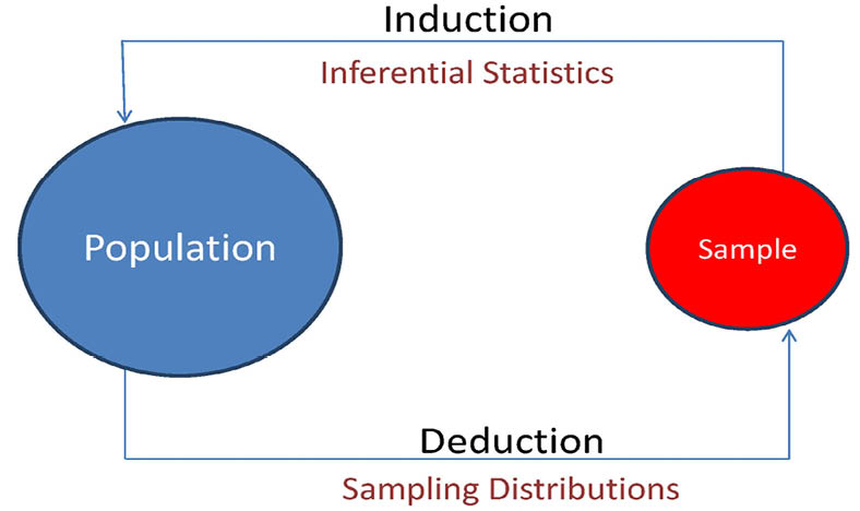
Ann Rigney has found that the average age in the sample of 100 was 44.16. In Chapter 5, we postulated that the standard deviation of the ages was 10 years. Using this, we calculated the standard error to be
This means that the margin of error is 2(1.00) or 2.00. Our 95% confidence interval then becomes
![]()
The margin of error requires a percentile from the test statistic which means that the confidence interval will depend on the nature of the sampling distribution. As we will see later, our discussion of statistical inference will mirror our discussions of sampling distributions in Chapter 5.
Finding the Right Sample Size
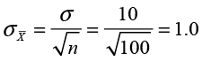
In the last chapter, we brought up the issue of how many elements of the population should we sample? We are now in a position to address that issue using the concept of margin of error. Putting our discussion above into formula terms, we have
 (6.3)
(6.3)
where E represents the margin of error and Z is a percentile from the standard normal distribution. With a little algebra we can rearrange the equation in terms of the sample size n as
 (6.4)
(6.4)
In other words, if we know the population standard deviation (σ), the degree of confidence we want (which determines Z), and if we can establish the margin of error that we want (E), we can solve the equation to find the required sample size to achieve this margin of error. For example, Ann had a margin of error of 2.0 with a sample size of 100. If she wants a margin of error of 1.0, how big a sample would she have to take?
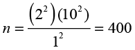
As you can see, she would have to take a much larger sample to achieve this margin of error. The JMP script accompanying the text will solve for the necessary sample size if you have the required information available.
Introduction to Hypothesis Testing
Estimation is a common task in inferential statistics. But often we already have an idea about the value of a population parameter based on past history, a particular theory, or the value of a reference group, and we would like to test that “hypothesis” to see if it is true or not. This is the basic idea of hypothesis testing. Hypothesis testing begins with the assumption that this hypothesis about the population is true and then, on the basis of the sample information, decide whether or not the hypothesis is still believable or not.
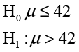
Hypothesis testing is conducted using two mutually exclusive and exhaustive hypotheses. The first is called the null hypothesis and is denoted as H0. The opposing hypothesis is called the alternative hypothesis and is designated as H1 (sometimes also symbolized as HA). For example, Ann Rigney has recently read an article in an industry publication that stated that the average age of credit union members is approximately 42 years old. Ann wonders if the membership in INCU is similar in age to the national average. She could formulate a hypothesis test as follows:
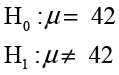
This version of the test is called a two-tailed hypothesis test. Alternatively, she could test to see if the membership in these two institutions is younger or older than the national average. These two alternatives are called one-tailed and would be formulated as
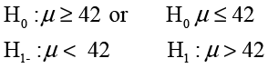
The first of these is called a lower-tailed test and the second an upper-tailed test. Notice that, in all three versions of the test, the two hypotheses are mutually exclusive and exhaustive. In other words, only one of them can be true, and one of them has to be true. Also notice that the equality sign is always in the null hypothesis. This must always be the case. In general, all hypothesis testing situations follow one of these three patterns.
To test these hypotheses, we gather sample data and on the basis of the value of the corresponding sample statistic, make a decision about whether or not the null hypothesis is true. If the sample data are consistent with the null hypothesis, we will accept that hypothesis;2 otherwise, we will reject the null hypothesis and conclude that the alternative hypothesis is true. But remember that we are dealing with inductive inference in this situation, and we may well be wrong when we make our decision. In terms of the true state of reality and the decision we make, we have four possible outcomes as shown in Figure 6.2.
Figure 6.2 Decision Outcomes in Hypothesis Testing
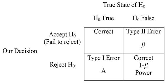
If the null hypothesis is true and we accept the null hypothesis, we have made a correct decision. Similarly, if the null hypothesis is false and we reject it, we have made a correct decision. However, if the null hypothesis is true and we reject the null hypothesis, we have made what is called a Type I error. The probability of making a Type I error is designated by the Greek letter α (alpha) and is called the level of significance. In traditional hypothesis testing, we establish the level of significance in advance, which by tradition is typically set at a small value such as .01 or .05. If the null hypothesis is false and we accept the null hypothesis (or fail to reject it), we have made a Type II error, which is designated by the Greek letter ß (beta). The correct decision to reject the null hypothesis when it is false is a special type of correct decision, and its probability is 1 – ß This is known as the power of the test. Since, as we will discuss shortly, what we want to demonstrate is in the alternative hypothesis, power is a measure of our ability to show what we are trying to demonstrate.
There is an inverse relationship between α and ß. The smaller we make the level of significance, the larger in general will be the probability of a Type II error. By using small values for the level of significance, we are biasing the process in favor of the null hypothesis. In general, we are more likely to accept a false null hypothesis (Type II error) than to reject a true null hypothesis (Type I error).
To understand this, an analogy with the Anglo-American criminal justice system is useful. In this system, the defendant is presumed innocent until proven guilty as shown in Figure 6.3.
Figure 6.3 Anglo-American System of Justice
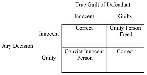
This system of justice is based on the premise that it is much worse to convict an innocent person than to let a guilty person go free. Therefore, the process is biased to reduce this type of error. Notice that convicting an innocent person corresponds to a Type I error in the hypothesis testing process. From everyday experience, we know that if a jury finds a defendant innocent, there is often a public perception that the person was really guilty but they just didn’t have enough evidence. In other words, judging a person innocent (accepting the null hypothesis) is not very convincing because of the bias in favor of the defendant. Similarly, accepting the null hypothesis on the basis of sample data is not very convincing. This is why some argue that we never “accept” the null hypothesis but merely fail to reject it. That is also why what we are trying to demonstrate must always be in the alternative hypothesis. Then if we can reject the null hypothesis, we have a strong argument for our claim. For this reason, the alternative hypothesis is sometimes called the research hypothesis as it contains what we are trying to demonstrate. In a business context, we will often take action or not depending on our decision about the hypotheses.3 Since we do not want to take action, which is usually costly, unless we are sure that the action will produce positive results, change always appears in the alternative hypothesis. Thus the alternative hypothesis is also sometimes called the action hypothesis.
But how do we make this decision about the null hypothesis? When do we decide that it is false? To illustrate the logic, we will use an example.
Example 6.2
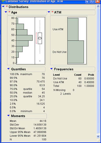
Ann Rigney is concerned that the members of INCU may be older than members of the average credit unit. Because she may take some marketing steps if she concludes that the members are older than average, she sets up the hypothesis tests as
In other words, she wants to make sure that they are in fact older on average before taking action. After we collect the data, values of the sample mean of 42 or below would support the null hypothesis, and values greater than 42 would support the alternative. However, since there is always sampling error, values that are above 42 but quite close to it (such as 42.1 or 42.5) are likely not strong evidence against the null hypothesis because this could just be sampling error. However, sample means of 50 or more would likely be strong evidence against the null hypothesis because values this large would not likely happen if the true mean is 42.
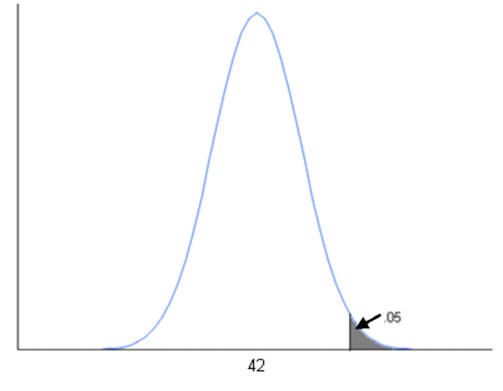
The question then is how large does the sample mean need to be before we conclude that the null hypothesis is false? The answer depends on the level of significance α and our knowledge of sampling error. Ann knows that the sampling distribution in this situation is a normal distribution; and if the null hypothesis is correct, the mean is equal to 42 or less. If we take the upper limit (the equality), then the mean is 42 and the standard deviation, which is the standard error, is 1.00 (see example 6.1). Now it is time to set our level of significance. Let’s use the traditional value of .05. The situation is as shown in Figure 6.4. As you can see, the value we need is the 95th percentile of the sampling distribution.
Figure 6.4 Setting a Critical Value for the Decision
We can use the Normal Quantile function to find this value. Using the function Normal Quantile (0.95, 42, 1.00), we get the results shown in Figure 6.5. The critical value is 43.65. If the sample mean is greater than 43.65, we will reject the null hypothesis, and, if it is less than 43.65, we will accept (not reject) the null hypothesis. As you may recall, Ann calculated the sample mean to be 44.16. So based on the sample data, we would reject the null hypothesis and conclude that the average age of the members of INCU is in fact older than the national average.
Figure 6.5 Critical Value for the Hypothesis Test

p-Values
Although the previous discussion is useful to understand the logic of hypothesis testing, it is not how testing is done in practice. In practice, analysts use p-values to make decisions about the null hypothesis. There are several advantages to using p-values.
- The decision rule is the same no matter whether the test is a two-tailed test, an upper-tail test, or a lower-tail test.
- The process is the same no matter what type of hypothesis is being tested.
- Virtually all statistical software, including JMP, routinely produces p-values as part of the output.
Whether you realize it or not, you are already familiar with p-values. Conceptually, a p-value is the probability of observing a sample statistic as extreme as the value observed if the null hypothesis is true. In other words, it is a probability from the sampling distribution similar to those we calculated in Chapter 5. If the observed p-value is less than the stated level of significance (α), then we reject the null hypothesis; if not, we accept (fail to reject) the null hypothesis. In Ann’s case, the p-value would be the probability of observing a sample mean of 44.16 or greater if the true population mean is actually 42. We can use the JMP Normal Distribution function to find this probability. Using the function input
Normal Distribution (44.16, 42, 1.00)
we would observe the probability shown in Figure 6.6. However, this is the probability of a value of 44.16 or less, and we want the probability of 44.16 or more. So we have to subtract this value from 1.0, which gives us a p-value of .0154. Since this p-value is less than .05, we can reject the null hypothesis just as we did before. Fortunately, JMP will produce these p-values for us so that we do not have to perform these calculations each time.
Figure 6.6 Calculation of the p-Value

Tests of Equivalence
As you may have noticed, all three of the hypothesis tests described in the last section are designed to show that a value is different from the hypothesized value. Because accepting the null hypothesis is not strong support because of the bias in favor of the null hypothesis, what we are trying to demonstrate is always in the alternative hypothesis. The three alternative hypotheses were
![]()
What if we want to show that the mean is equal to 42; i.e., what if we really want to show that the traditional null hypothesis is true? Such situations arise often in medical science but are also common in a business environment. For example, engineers might devise a new process that promises to lower the variability of a process but leave the average value the same. Demonstrating that the variance of the new process is less than that of the old process is straightforward using traditional hypothesis tests. But what about showing that the new process has the same mean as the old process? This would be proving the null hypothesis, which is counter to traditional practice. The solution is equivalence testing.
To illustrate the logic, let’s go back to Ann’s situation with the customer survey. The article that Ann read also stated that the average tenure of members in credit unions nationally is 10 years. Ann believes that the members at INCU are typical in this regard and would like to demonstrate this using the sample data. In effect, what Ann would like to do is
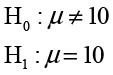
However, traditional hypothesis testing requires that the equality appear in the null hypothesis. A little reflection should convince you that what Ann really wants to show is not that the mean is exactly 10.0000 but that there is really no practical difference between members at INCU and other credit unions across the nation—in other words, that there is no practical difference between the mean and 10. If we can define the notion of practical difference numerically, then it is possible to demonstrate that the mean is, for all practical purposes, 10 years. We will call the small numerical value of µ the practical difference value δ. Then what we want to demonstrate is that the population mean µ is between 10 - δ and 10 + δ. We can do this with two hypothesis tests.
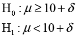
and
The first test, if we reject H0, shows that the mean is < 10 + δ; and the second, again if we reject H0, shows that it is > 10 – δ, which implies that it must be between the two values. Since this involves two one-sided hypothesis tests, this procedure is often referred to as Two One-Sided Tests or TOST.4
JMP and Inferences about One Variable
To illustrate the application of statistical inference in JMP, we will consider only inferences about one variable at a time in this chapter, the so called univariate analysis. The remaining chapters of the text will consider the simultaneous analysis of more than one variable.
How we analyze variables in JMP depends on the type of variable we are dealing with. In particular, it depends on whether the variables are nominal scale, ordinal scale, or continuous (interval or ratio scale) variables. To illustrate the analyses, we will use the customer survey that Ann Rigney is analyzing. The basic structure of the data is shown in Figure 6.7.
Figure 6.7 Customer Survey Data Table

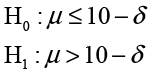
In the rest of this chapter, we will use the columns Age and ATM to illustrate the basic principles of statistical inference in JMP. To perform a univariate analysis, we use the Distribution platform in JMP. After opening the Customer Survey.jmp data table, Ann selects Analyze → Distribution from the JMP menu and in the dialog selects Age and ATM as the Y, Columns in the Distribution dialog as shown in Figure 6.8.
Figure 6.8 Completed Distribution Dialog
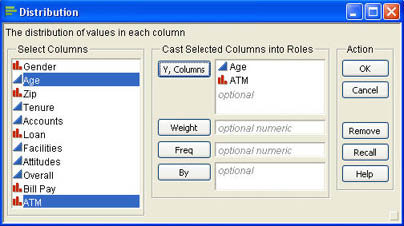
After clicking OK, she views the results shown in Figure 6.9. As you can see from the graphs of the Age column, it appears to be somewhat negatively skewed, and there is one outlier in the lower end of the age distribution. We can also see this in that the mean (44.16) is less than the median (45). The standard deviation of the ages in the sample is approximately 14.66. For the ATM variable, we can see that 40 out of the 100 members sampled (40%) reported that they used the ATMs while 60% did not. In the following sections, we will illustrate the use of JMP to go beyond the descriptions of the sample to make inferences about the population on the basis of the sample data.
Inferences about Means
We will first consider inferences about means for continuous (interval or ratio scale) quantities such as age. Recall from the last chapter that the sampling distribution for the sample mean is either a normal distribution if we know the population standard deviation, or the Student t-distribution if we do not know σ. We will need that information to make inferences about the mean. Going back to the analysis for Age in Figure 6.9, we note that the sample mean is 44.16 with a standard deviation of 14.66.
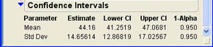
The standard error of the mean (Std Err Mean) is 1.46. Below the standard error, JMP displays the confidence interval for the population mean. The interval is from 41.25 to 47.07. This interval is wider than the interval we previously computed because the standard error is larger. In Example 6.1, we assumed a population standard deviation of 10, which gave us a standard error of 1.0. However, here we are assuming that we do not know the population standard deviation, so we use the sample standard deviation to compute the standard error and get a larger standard error of 1.46.
JMP automatically supplies the 95% confidence interval for the mean whenever we use the distribution platform to analyze a continuous variable. What if you want a different degree of confidence? Also, this confidence interval assumes that you do not know the population standard deviation and uses the t-distribution. Although this is the most common situation, sometimes you may know the population standard deviation and want to use the normal distribution. To vary the nature of the confidence interval, you need to use the distribution platform options. Click the drop-down menu next to age (![]() ) in the report to access the options menu shown in Figure 6.10. Select Confidence Interval to produce the submenu shown in Figure 6.10. Here you can select a different degree of confidence. If the desired degree of confidence is not one of those shown, click Other. This will produce a dialog like that shown in Figure 6.11.
) in the report to access the options menu shown in Figure 6.10. Select Confidence Interval to produce the submenu shown in Figure 6.10. Here you can select a different degree of confidence. If the desired degree of confidence is not one of those shown, click Other. This will produce a dialog like that shown in Figure 6.11.
Figure 6.10 Distribution Platform Options
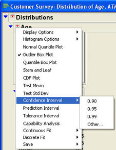
Figure 6.11 Dialog to Set Degree of Confidence or Value of σ

You can either enter a different confidence level, choose to do a one-sided confidence interval, or indicate that the population standard deviation is known. To indicate a known standard deviation, check the Use known Sigma box. When you do this, you will be prompted to enter a value for σ. If you use any of these options, the new confidence interval will be shown below the Moments section of the report.
Although the confidence intervals are produced automatically, testing a hypothesis requires that you use the Distribution options. In Figure 6.10, there is a Test Mean option. When you select this option, you will see the dialog shown in Figure 6.12.
Figure 6.12 Test Mean Dialog
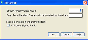
To test a hypothesis about the mean enter the hypothesized value in the Specify Hypothesized Mean box. If you know the population standard deviation and should use the normal distribution, enter the value of the true population standard deviation into the appropriate box otherwise leave that box blank.
Example 6.3
To illustrate the test for means, let’s go back to Ann Rigney’s situation in Example 6.2. Ann wanted to know whether INCU’s members were older on average than the average national credit union member at 42 years old. To test the hypothesis in JMP, Ann clicks the drop-down menu next to age (![]() ) in the report to access the options menu previously shown in Figure 6.10 and selects the Test Mean option. She enters 42 for the hypothesized mean. Since she knows that the population standard deviation is 10, she enters that value in the appropriate box and clicks OK. The results shown in Figure 6.13 are displayed at the end of the Age results window. The first value is the value of the Z test statistic, which, as we discussed in the last chapter, is calculated as
) in the report to access the options menu previously shown in Figure 6.10 and selects the Test Mean option. She enters 42 for the hypothesized mean. Since she knows that the population standard deviation is 10, she enters that value in the appropriate box and clicks OK. The results shown in Figure 6.13 are displayed at the end of the Age results window. The first value is the value of the Z test statistic, which, as we discussed in the last chapter, is calculated as
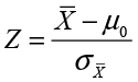
where µ0 is the hypothesized population mean, in this case 40. Following the test statistic, three p-values are displayed. The p-value labeled Prob > |Z| is the p-value for the two-tailed hypothesis test. The p-value labeled Prob > Z is for the upper-tailed test, and the value labeled Prob < Z is for the lower-tailed test. Since Ann was performing an upper-tailed test, she notes that the relevant p-value is .0154, which agrees with our earlier calculations. Therefore, Ann can reject the null hypothesis and conclude that her members are indeed older than those of the average credit union.
Figure 6.13 Results of the Test Mean for Age
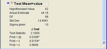
You may note that the two-tailed p-value is exactly twice the value of the smaller of the two one-tailed values. This is not a coincidence. To find the two-tailed p-value, JMP multiplies the smaller of the two one-tailed p-values by 2. This has important consequences. It means that you are always more likely to reject the null hypothesis with a one-tailed test. In other words, a one-tailed test is more powerful than a two-tailed test. If there is a logical reason for a one-tailed test, you should always use it rather than a two-tailed test.
Inferences about Variances and Standard Deviations
JMP also allows you to make inferences about variances or standard deviations. Although, as we saw in Chapter 5, there is no known sampling distribution for the standard deviation, we can make the appropriate inferences about the variance by making the appropriate adjustments. JMP handles these details for us.
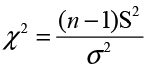
Recall from Chapter 5 that the sampling distribution for the variance is the chi-square distribution if the population follows a normal distribution. When JMP produces confidence intervals or performs hypothesis tests about a standard deviation, it automatically converts the values to variances, performs the calculations for the chi-square distribution, and then converts the results back to standard deviation units.
To obtain a confidence interval for the standard deviation, click the drop-down menu next to age (![]() ) in the report to access the options menu previously shown in Figure 6.10 and select the Confidence Interval option. You can select one of the standard degrees of confidence as shown in Figure 6.11 or insert your own value. When you click OK, JMP will calculate confidence intervals for both the mean and standard deviation and show the results at the bottom of the Report window. They should look like those shown in Figure 6.14. As you can see, the lower limit of the 95% confidence interval for the population standard deviation is 12.87, and the upper limit is 17.03. If you want a confidence interval for the variance, simply square the values shown for the standard deviation.
) in the report to access the options menu previously shown in Figure 6.10 and select the Confidence Interval option. You can select one of the standard degrees of confidence as shown in Figure 6.11 or insert your own value. When you click OK, JMP will calculate confidence intervals for both the mean and standard deviation and show the results at the bottom of the Report window. They should look like those shown in Figure 6.14. As you can see, the lower limit of the 95% confidence interval for the population standard deviation is 12.87, and the upper limit is 17.03. If you want a confidence interval for the variance, simply square the values shown for the standard deviation.
Figure 6.14 Confidence Interval for the Standard Deviation
Hypothesis tests for the standard deviation are performed in much the same way as hypothesis tests for the mean.
Example 6.4
Since Ann has discovered that the members of INCU are older on average than those at other credit unions, she also wonders if there is a difference in the variability of the ages at INCU compared to those at other credit unions. The report stated that the standard deviation of ages is 10 years. Ann wants to test the hypothesis that the standard deviation at INCU is the same as the national value.
H0: σ = 10
H1: σ ≠ 10
To test the hypothesis, Ann clicks the drop-down menu next to age (![]() ) in the report to access the options menu previously shown in Figure 6.10 and selects the Test Std Dev option. JMP then asks for the hypothesized population standard deviation as shown in Figure 6.15. After entering the value of 10, Ann clicks OK, and the results shown in Figure 6.16 are added to the bottom of the Results window.
) in the report to access the options menu previously shown in Figure 6.10 and selects the Test Std Dev option. JMP then asks for the hypothesized population standard deviation as shown in Figure 6.15. After entering the value of 10, Ann clicks OK, and the results shown in Figure 6.16 are added to the bottom of the Results window.
Figure 6.15 Dialog for Hypothesis Tests for the Standard Deviation
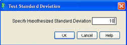
Figure 6.16 Hypothesis Testing Results for the Standard Deviation
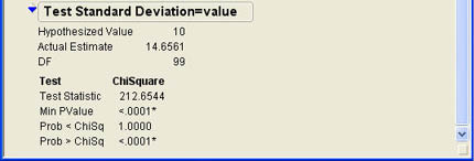
Similar to the hypothesis test for means, JMP first prints the summary measures and then displays the value of the test statistic. In this case, the test statistic is the chi-square statistic as described in Chapter 5.
The results show p-values for both one-tailed tests. The results do not directly show the two-tailed p-value, but you can get it by multiplying the Min PValue probability by 2. In this case, the relevant p-value is .0002. Therefore, Ann can reject the null hypothesis and conclude that the ages at INCU are more variable than those at the typical credit union.
Inferences about Medians
The statistical theory on medians is not as well developed as it is for means, proportions, and variances. As we discussed in Chapter 5, there is no general sampling distribution for medians. As we will see in later chapters, there is often confusion about what some of the tests for medians are really testing. At this point, we will introduce a simple test for one median that can be performed using JMP and inferences based on the bootstrapping concept introduced in Chapter 5.
Sign Test for Medians
The sign test is not included directly in JMP, but the test is easy to understand and can be easily computed using JMP. We will illustrate the sign test in the context of an example.
Example 6.5
Mary Warner, the Chief Operating Officer (COO) at INCU is concerned with the quality of services provided at INCU and how those services are perceived by the customers. She wants to use the three quality related questions asked on the customer survey to get a better understanding of how their customers perceive the quality of the services at INCU. She decides to start with the overall quality rating, the Overall column in the data. This variable is measured on a 7-point scale with 4 being a neutral point, values below 4 indicating negative perceptions about quality, and values above 4 indicating positive perceptions. Mary decides to start with the question of whether or not the median ratings are positive—i.e., greater than 4.
H0:η ≤ 4
H1: η > 4
The sign test uses the basic fact that the median is the middle value. Therefore, if the hypothesized value (η = 4) is true, then about half of the sample values should be less than 4 and half should be greater than 4. Values exactly equal to 4 are omitted from the count. We can then use the binomial distribution to see if this hypothesis is true.
Mary first right-clicks the header of the Overall column in the data table and selects Sort, which sorts the data based on the overall quality rating as shown in Figure 6.17.
Figure 6.17 Data Sorted on Overall Quality Rating
Scrolling down, Mary notes that the “4” ratings end with the 41st observation. This means that 41 out the 100 customers surveyed rated the overall quality as 4 or less, which implies that 59 rated the overall quality as higher than 4. If we count a quality rating higher than 4 as a “success,” we have 59 successes out of 100 trials of a binomial problem where the probability of a success should be .5 according to the definition of a median and our null hypothesis. We can then calculate the p-value using the binomial function in JMP. Mary creates a new column in the data table and labels it “P-value.” The p-value is the probability of observing 59 successes or more in 100 trials if the probability of a success is .5. Since the Binomial Distribution function returns a cumulative probability, Mary knows she should find the cumulative probability of 58 or fewer successes and then subtract from 1.0. She enters the following formula into the column:
Binomial Distribution (0.5, 100, 58)
The formula result is shown in Figure 6.18, which is a probability of .9557. Subtracting this from 1.0 gives a p-value of .0443. Since this is less than .05, we can reject the null hypothesis and conclude that the median overall quality rating is positive—i.e., greater than 4.
Figure 6.18 Binomial Distribution Calculation Results

Bootstrapping Inference about the Median
The problem with the sign test is that it is not a very powerful test. Although the results turned out to be statistically significant in Mary’s test, it is still desirable to have a more powerful test. Bootstrapping gives us such an option.
The supplementary JMP script (available as a download from the author’s Web site at http://support.sas.com/publishing/authors/index.html) will perform confidence intervals and perform hypothesis tests for medians utilizing bootstrapping. The basic ideas of statistical inference using bootstrapping are straight forward.
Confidence Intervals Using Bootstrapping
Recall that bootstrapping generates an empirical sampling distribution based on resampling from the original sample. We also know that the confidence intervals are basically the appropriate percentiles of the sampling distribution for the sample statistic. Putting these two ideas together, a confidence interval for the median will be the appropriate percentiles from the bootstrapped sampling distribution. For example, for a 95% confidence interval, this would be the 2.5th percentile and the 97.5th percentiles. If we generated 1000 samples in our bootstrapped distribution and sorted the resulting medians from lowest to highest, the 25th and 975th values would be the lower and upper limits of the confidence interval. Using the JMP script, the 95% confidence interval for the median age from our customer survey would be from 42 to 48 years.5
Hypothesis Testing Using Bootstrapping
Using bootstrapping for hypothesis testing is conceptually similar to its use for confidence intervals. We have defined the p-value as the probability of observing a sample value this extreme if the null hypothesis is true. However, the bootstrapping should be done assuming that the null hypothesis is true. The simplest way to do this is to adjust the values in the sample by the difference between the hypothesized value and the observed sample value.6 Then, given the bootstrapped sampling distribution we simply need to determine the proportion of the values that are as large (small) or larger (smaller) than the observed value to get the p-value. Our decision about the null hypothesis follows the familiar logic after obtaining the p-value.
Using the JMP script to calculate the p-value for Example 6.5 shows that the resulting p-value is .0001, and we can safely reject the null hypothesis.
Inferences about Proportions
Proportions are appropriate measures for nominal variables where the analysis is based on frequencies or counts. A proportion is simply the frequency with which a value occurs in the data divided by the number of observations in the data table. To illustrate statistical inferences for nominal variables, we will return to the INCU customer survey.
Example 6.6
Ann Rigney has a sense that the ATMs are not being used as much as they should be by INCU members. She wants to analyze the ATM use question in the customer survey to get a better idea of how much their members use the ATMs and how this compares to other credit unions. The responses to the ATM question are contained in the ATM column of the data. Ann decides to use the Distribution platform to get a feel for the data. She selects Analyze → Distribution. In the JMP menu, she selects ATM from the list of columns and clicks Y, Column to add it to the columns to be analyzed and then clicks OK. The results are shown in Figure 6.19.
Figure 6.19 Distribution Platform Results for ATM Use
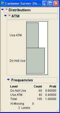
Ann quickly sees that 40 out of 100 members surveyed use the ATMs, which is a proportion of 40%. This is her best estimate then of the proportion of all INCU members that use the ATMs. Ann would like to get a confidence interval estimate to see how much sampling error there is in the estimate. Ann clicks the drop-down menu next to ATM (![]() ) in the report to access the options menu shown in Figure 6.20.
) in the report to access the options menu shown in Figure 6.20.
Figure 6.20 Distribution Platform Options for Nominal Columns
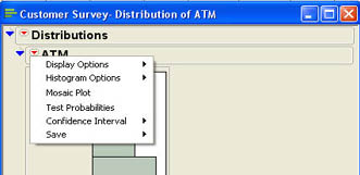
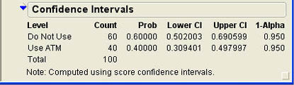
She selects Confidence Interval from the options, which leads to the same submenu of choices as when setting the level of confidence for means shown in Figure 6.10. She selects 95% for the confidence interval, and the results shown in 6.21 are appended to the report. From the results, she can see that the confidence interval for the proportion ranges from 30.9% to 49.8%. Therefore, she can be quite confident that a majority of her members do not use the ATMs at INCU.
Figure 6.21 Confidence Interval Results for ATM Use
Ann recently found a study on a Web site that indicated that approximately 45% of customers at financial institutions nationwide use the available ATMs for at least some transactions. Ann wonders if the 40% usage she found in her sample indicates a significantly lower ATM usage rate at INCU. In other words, Ann wants to test the following hypotheses:
H0: π ≥ .45
H1: π < .45
To perform the hypothesis test, Ann clicks the drop-down menu next to ATM (![]() ) and selects Test Probabilities from the options shown in Figure 6.20. The dialog shown in Figure 6.22 is added to the results window.
) and selects Test Probabilities from the options shown in Figure 6.20. The dialog shown in Figure 6.22 is added to the results window.
Figure 6.22 Test Probabilities Dialog
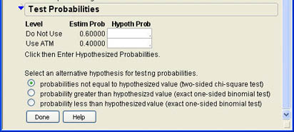
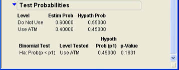
Ann first enters the hypothesized proportions in the boxes under the label Hypoth Prob. She enters .55 for Do Not Use and .45 for Use ATM. She then needs to choose whether to use a two-tailed test, an upper-tailed test, or a lower-tailed test. The one-tailed tests use the binomial distribution since, as we saw in the last chapter, the correct sampling distribution for proportions is the binomial distribution. The two-tailed test used a chi-square test. (This is a different use of the chi-square distribution that we will examine in more detail in Chapter 7.) Since Ann’s test is a lower-tailed test, she selects the last option and clicks Done. This portion of the results section then changes to look like that shown in Figure 6.23. The figure shows that the p-value is .1831, which is not less than .05 so we cannot reject the null hypothesis and conclude that there is not sufficient evidence that the INCU members differ from the national average in terms of ATM usage.
Figure 6.23 Results of the Hypothesis Test for Proportion
Finding the Right Sample Size for Proportions
The logic in finding a required sample size for proportions is the same as for the mean. For proportions the margin of error is
 (6.5)
(6.5)
Again, we can solve this equation for n to find
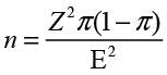 (6.6)
(6.6)
An additional complication here is that you have to have a value of the parameter you are trying to estimate to find the required sample size. If you have a prior estimate of π, it can be used in Equation 6.6. A conservative approach is to use a value of .5 for i;, which gives you the largest possible sample size. If the sample proportion turns out to be different from .5, then the sampling error will be somewhat smaller.
Ann found that she had a margin of error of .10 in her sample of 100 (see Figure 6.21). Thinking that this was rather large, she wondered what size sample she would need to get a margin of error of 3%.

Ann would need a sample of around 1,000 or so to achieve this margin of error.7 Notice that we seem to need much larger samples for proportions than we did for means. This is true in general because there is much less information in a nominal variable than there is in a continuous variable.
Summary
This chapter introduces the basic logic of statistical inference, which is based on the sampling distributions introduced in Chapter 5. Statistical inference can be divided into estimation and hypothesis testing. Estimation involves both point estimates and interval estimates.
The concepts of nonsampling and sampling error are introduced in this section. Sampling error, more commonly called the margin of error, is the standard error along with a percentile from the test statistic for the sampling distribution, reflecting the likelihood for the desired degree of confidence. The standard error, introduced in Chapter 5, is simply the standard deviation for the sampling distribution of the sample statistic. An interval estimate centers the margin of error around the sample statistic to obtain a confidence interval with the desired degree of confidence.
A hypothesis is a statement about specific values of the population parameter. Hypothesis testing involves testing a specific hypothesis to see if these are the true values or not. A hypothesis test involves two hypotheses: a null hypothesis (H0), which always contains an equal sign for an exact value; and the opposite hypothesis, called the alternative hypothesis (H1). Hypothesis tests can be two-tailed, lower-tailed, or upper-tailed tests. When a hypothesis is tested, two errors can occur. A Type I error is rejecting the null hypothesis when it is true. A Type II error is accepting a null hypothesis when it is false. In practice, a Type I error is regarded as the more serious error, and the traditional hypothesis testing process is biased in favor of the null hypothesis to guard against this type of error. Because of this bias, what we want to demonstrate should always be in the alternative hypothesis. Equivalence testing was also introduced in this chapter. Demonstrating that a population parameter is approximately equal to a specific value, normally contained in the null hypothesis, can be done using two one-sided tests or TOST.
Statistical inference for a single variable in JMP uses the Distribution platform, but the details vary depending on the nature of the variable involved (nominal, ordinal, or continuous) and the specific sample statistic (mean, standard deviation, median, or proportion). Inferences about means, standard deviations, and variances can be made directly within JMP. Inferences about medians require the use of a JMP script and bootstrapping.
Chapter Glossary
- alternative hypothesis (H1)
- The opposite of the null hypothesis that contains what the analyst is trying to demonstrate or the case for taking action.
- confidence interval
- An interval bounded by a lower bound and an upper bound such that we are confident that the population parameter falls inside that interval with a particular degree of confidence.
- equivalence testing
- Reverses the hypothesis testing procedure to demonstrate what is traditionally the null hypothesis, that the population parameter is equivalent to a particular value.
- hypothesis testing
- The process of deciding which of two mutually exclusive and exhaustive hypotheses about a population parameter are best supported by the data.
- level of significance (α)
- The risk that the analyst is willing to take of making a Type I error.
- margin of error
- A measure of sampling error that includes the standard error along with a percentile from a test statistic.
- nonsampling error
- Error introduced by how the statistical study is conducted or during the data recording and processing phase. Often results in systematic error or bias.
- null hypothesis (H0
- The hypothesis that is explicitly tested in the hypothesis testing process. This hypothesis is assumed to be true unless proven false by the data.
- power
- The opposite of a Type II error, this value indicates our ability to correctly reject the null hypothesis when it is false.
- p-value
- The probability of observing a value of the sample statistic as extreme as the value observed in the data if the null hypothesis is true. Compared with the level of significance to make a decision about the null hypothesis.
- sampling error
- Error that causes the sample statistic to be different from the population value because the sample is not perfectly reflective of the entire population.
- two one-sided tests (TOST)
- Two one-sided hypothesis tests that are used in equivalence testing to demonstrate that the population parameter is approximately equal to a specific value.
- unbiased estimator
- A sample statistic used to estimate a population parameter whose sampling distribution has a mean equal to the population value being estimated.
- univariate analysis
- The analysis of one variable at a time.
Questions and Problems
Hank Wilson, the CFO at INCU, wants to know whether or not INCU members use the Internet-based bill-paying option at the INCU Web site. Using the Customer Survey.jmp data, answer the following questions:
1. Develop a 95% confidence interval for Hank Wilson for the proportion of all INCU members who use the bill pay facility.
2. Do more than 15% of the INCU members use the bill pay option? Conduct a hypothesis test to support your conclusions.
3. Hank would also like to know what percentage of INCU customers currently have a loan with INCU. What can you tell him about this issue?
Ann Rigney has read that the average number of accounts per member at a typical credit union is 2.5 accounts.
4. How do the number of accounts per member at INCU compare with the typical credit union? Support your conclusions with statistical inference.
5. Ann would also like to know if the mean quality ratings for facilities and for attitude of the employees are significantly greater than neutral (a rating of 4.0). What can you tell her about this? Support your conclusions with data and statistical inference.
6. Ann is also curious whether there is an even split between male and female members at INCU or if one or the other gender tends to dominate. What can you tell her based on the survey data?
References
Wellek, Stephan. 2003. Testing Statistical Hypotheses of Equivalence. Boca Raton, FL: Chapman & Hall.
Ramirez, Jose.G., and Brenda S. Ramirez. 2009. Analyzing and Interpreting Continuous Data Using JMP: A Step-by-Step Guide. Cary, NC: SAS Institute Inc.
Notes
1 You often hear the term margin of error used in conjunction with public polls on the news.
2 Some will argue that you do not accept a null hypothesis but merely fail to reject it. This is because of the bias in favor of the null hypothesis in the usual practice of hypothesis testing. The classic hypothesis testing procedure first articulated by Sir Ronald Fisher, however, clearly stated the decision as a strict dichotomy—you either accept or reject the null hypothesis. We will not make too much of this distinction either way in this text.
3 For example, stop a process to fix it if it is out of control, or adopt a new process if it is better than the old one, or make changes if they appear to produce better results.
4 For more information about equivalence testing, see Wellek (2003) or Ramirez and Ramirez (2009). Ramirez and Ramirez have also written a short article on the process for JMPer Cable magazine (Winter 2010) available at JMP.com.
5 Your results may vary somewhat because of the random resampling process but should be close to the results given here.
6 This adjustment process assumes that the bootstrapped sampling distribution has the appropriate shape and the correct variance but only differs in scale from the true population.
7 You may notice that sample sizes of 1,000 are very common in opinion polls. This is not an accident. This sample size gives a margin of error of about 3%.
..................Content has been hidden....................
You can't read the all page of ebook, please click here login for view all page.