Up to this point in the text, we have looked primarily at one variable at a time. The lone exception was in Chapter 3 where we looked at multiple variables in tables and graphs. In this section, we will examine the impact that one variable has on another and will return to some of the graphical displays that we discussed earlier. Most of the discussion in this section will involve a single platform, the Fit Y by X platform. This chapter will look at the impact of a qualitative variable on a quantitative variable. In standard statistics texts, the topics in this chapter would go under the headings of tests of two groups and analysis of variance (ANOVA). One difference you may notice in this chapter is that we will deal only with means, variances, and medians and will not discuss proportions. That is because this chapter deals only with the impact of a qualitative variable on a quantitative variable. We will deal with the impact of a qualitative variable on another qualitative variable in the next chapter.

The Situation at INCU

Mary Warner, the Chief Operating Officer, is concerned about waiting times in some of the larger branches at INCU. Waiting lines form at the teller windows and also sometimes for loan officers. Mary has some ideas on structural and procedural changes that she would like to try to see if some of the waiting times can be reduced. She has asked Bill Williams, the Director of Member Services, to help with this project.

One of Bob Reed’s responsibilities in Human Resources is in terms of compliance with the Equal Employment Opportunity Act or discrimination. Bob has to monitor things such as salary, hiring, and firing decisions to make sure that there is no discrimination with regard to gender, race, or disabilities.

Ann Rigney is still concerned about the quality ratings in the customer survey and what factors impact these ratings. She wants to explore some of the other factors such as gender, use of ATMs, and other qualitative variables that may influence these ratings.

Qualitative Variables and Grouping

By qualitative variables we mean primarily nominal scale variables in this chapter. Since nominal variables contain only information indicating that objects differ in some way, the primary use of such variables is to divide observations into groups. Therefore, looking at the impact of a variable like gender on salary is the same as asking about the differences in salary between the two groups designated male and female. At times, we will use terminology suggesting the impact of a qualitative variable on another variable, and at other times will talk about the differences between groups. You should be aware that these are simply different ways of looking at the same phenomena.

Historically, material dealing with two groups has been treated separately from that of three or more groups. Part of this separation is because of the historical development of the field of statistics, and part is because of subtle differences between the two situations. We will maintain this separation in this chapter, but you will see considerable overlap between the two areas.

Independent and Dependent Variables (Factor and Response)

There is another way to view the qualitative variable in this chapter. We will introduce the Fit Y by X platform of JMP where we look at the impact of one variable (X) on another variable (Y). In traditional terms, X is usually called the independent variable, and Y the dependent variable because its value “depends” on the value of X. In JMP, the independent variable is called the Factor, and the Y variable is called the Response. Although we will often talk about the differences between groups in this chapter, we could usually just as well talk about the impact of the Factor (independent variable) on the Response (dependent variable). For example, we can talk about the differences between males and females in their perceptions of quality or talk about the effect of gender on perceptions of quality. We will do both interchangeably in this chapter and the next.

Independent versus Dependent Groups

There is an important distinction that impacts how we model the effect of a qualitative variable on another variable. That distinction is between independent groups and dependent groups. Independent groups are when the objects in the two groups created by the qualitative variable are independent or unrelated to one another. For dependent groups, the objects in the groups are related in some way. Such groups are said to be correlated. There are two different situations where dependent groups can arise.

When the objects are the same objects in both groups. This commonly occurs in before-after experiments when objects are measured before an event or experimental treatment and then again after the treatment or event.
When the objects in the different groups are matched or paired on the basis of some characteristic.

In Chapter 1, we discussed the distinction between experiments and post-hoc studies. As you might gather from the descriptions, dependent groups occur most often in an experimental context where the analyst has active control and has the ability to match or pair objects. Such situations are rare in post-hoc studies.

The distinction between dependent and independent groups is important because the way in which we analyze the data depends on which type of group we have. As we will see later, there are also important differences in the power of the two types of tests. In general, tests of dependent groups are more powerful than tests of independent groups.

Qualitative Variables with Two Levels

We will begin with qualitative variables that have only two levels or values so that the tests are for the differences between two groups. We will discuss both independent and dependent groups.

Independent Groups

Independent groups are analyzed with the Fit Y by X platform of JMP. You can access this platform either through the JMP Starter or through the JMP menu. Using the JMP Starter, you can access this platform through the Basic group as shown in Figure 7.1.

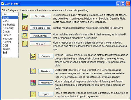
Figure 7.1 Accessing Fit Y by X via JMP Starter

The Fit Y by X platform really consists of four different types of analyses, depending on whether Y is qualitative or quantitative and whether X is qualitative or quantitative. The four types are labeled Oneway, Bivariate, Contingency, and Logistic. If you know which type of analysis you want, you can click directly on one of these options. Most of our work in this chapter will be done within the Oneway option. Optionally, you can click Fit Y by X, and JMP will automatically determine the type of analysis depending on the nature of the columns you pick to analyze.

You can also select Analyze → Fit Y by X from the JMP menu, which is the same as clicking Fit Y by X in the JMP Starter. In either case, you will see the dialog shown in Figure 7.2. You may have noticed the four icons in the lower-left portion of the dialog representing the four types of analyses just discussed. These are not clickable buttons; they merely indicate that JMP will decide on the appropriate analysis type depending on the nature of the columns you pick. In this chapter, we will be dealing with qualitative X variables and quantitative Y columns, both of which use the Oneway analysis. In the next chapter, we will deal with qualitative X variables and qualitative Y variables, both of which use the Contingency option. In Chapter 9, we will deal with quantitative X variables and quantitative Y variables, both of which utilize the Bivariate option. The final option, the Logistic option, examines the impact of a quantitative variable on a qualitative variable and will be covered in Chapter 10.

Figure 7.2 Fit Y by X Dialog

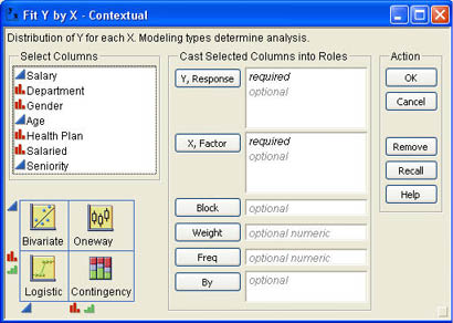
To perform an analysis, select the quantitative Y columns you want to analyze and click Y, Column. Then select the qualitative X columns you want and click X, Factor. Then click OK to start the analysis.¹

Example 7.1

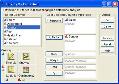
Since Bob Reed has the sample data on employees at INCU discussed in Chapter 3, he decides to do a quick check on salaries by gender to make sure that there are no problems with regard to possible pay discrimination. Loading the data table Employee Data.jmp he selects Analyze → Fit Y by X from the JMP menu. In the dialog he selects Salary as the Y Column and Gender as the X, Factor as shown in Figure 7.3. When he does this Bob notices that JMP has automatically selected the OneWay analysis as indicated under the column list in Figure 7.3. After he clicks OK he observes the results shown in Figure 7.4. The initial results for the Fit Y by X platform are a simple dot plot of the observations grouped by the X, Factor selected. Bob can see immediately that the male salaries tend to be higher overall than the female salaries. The male salaries also seem to be more spread out or variable. There are a variety of reasons why this might be true besides discrimination.

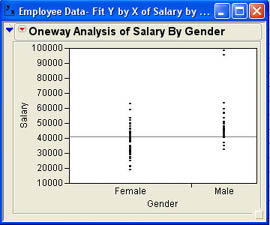
Figure 7.3 Fit Y by X Dialog for Example 7.1

Figure 7.4 Initial Results for Example 7.1

For example, the salary differences could be due to seniority differences, departmental differences, or other factors. Bob makes a quick note to investigate some of these other factors later. For now, Bob wants to make sure that the results are not just from sampling error. To do this, he needs to perform hypothesis tests to determine if the differences in salaries are statistically significant and not just sampling error.

Tests for Two Means

Bob first wants to know if the difference between the average salaries is significantly different from zero. The null and alternative hypotheses are

H₀: µ₁= µ₂ or H₀: µ₁ − µ₂= 0

H₁: µ₁≠ µ₂ H₁: µ₁− µ₂= 0

The second form of the hypotheses is more general in that it allows you to test for any difference, not necessarily zero.² The first form is by far the most commonly used because in most situations our concern is whether or not the means are the same or different. To perform the hypothesis test, Bob needs to use one of the options in the results window. Bob clicks the drop-down menu () next to the One Way Analysis of Salary by Gender in the report to access the options menu shown in Figure 7.5.

Figure 7.5 Options for the Oneway Analysis

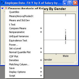
There are a variety of options available for this analysis, but here we will cover only the most important for our purposes. The option Bob wants at this point is the Means/Anova/Pooled t option. After he selects this option, the results window changes as shown in Figure 7.6. For simplicity at this point, the Summary of Fit and Analysis of Variance sections of the report have been closed. These sections will be covered in detail later when we discuss three or more groups.

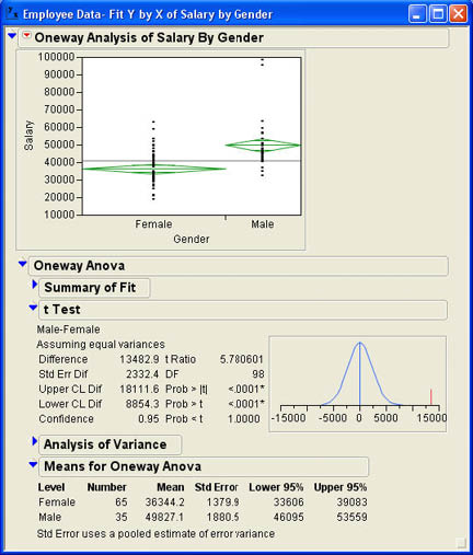
Figure 7.6 Oneway Results for the Salary by Gender Analysis

Notice that mean diamonds have been added to the plot. The line through the middle of each diamond represents the mean for that group. The height of the diamond represents the confidence interval for the mean. If these confidence intervals do not overlap, as is the case here, that is an indication that there is a significant difference between the two groups.

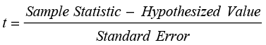
Our main focus here is on the t Test and Means for Oneway Anova sections of the report. From the Means section of the report, you can see that there are 65 females and 35 males in the sample and that the average salary for females is $36,344.20 and for males is $49,827.10. The difference between the two sample means is $13,482.90. This difference is certainly greater than the 0 difference that is hypothesized for the population. The question remains, is this difference statistically significant; i.e., can we reject the null hypothesis? To determine this, we must look at the t-test results. It will help at this point to review the t-test statistic. As we described it in Chapter 5 (Equation 5.11), the t-test statistic was

Image7508.EPS

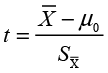
where µ₀ is the hypothesized value of the population mean and S_X is the standard error of the mean. As we will see many times in the text, this is the standard form of the t-test statistic which can be put in generic format as

Image7527.EPS (7.1)

For the difference between two groups, the sample statistic is (X ₁−X ₂) and the hypothesized value is (μ₁−μ₂)which is normally zero under the null hypothesis. There are two different forms of the t-test for two groups, which differ in the way the standard error and degrees of freedom are calculated. One of the tests, the one performed here, assumes that the population variances are equal. As you can see here, the results section states Assuming equal variances at the top. If we assume that the variances in the population are equal, then we can average the two sample variances to get a better estimate of the population variance. The standard error is then based on this pooled estimate of the variance as stated at the bottom of the report. The degrees of freedom for this test are n₁ + n₂ – 2. You may also notice the message at the bottom of the report that the standard error uses a pooled estimate of the variance.

Going back to the t Test section of the report, we see that the difference between the sample means (Difference) is 13482.9, as we noted before. The standard error of the difference (Std Err Dif) is 2332.4. Dividing the difference between the means by the standard error gives a t value (t Ratio) of 5.78061. The degrees of freedom (DF) are 65 + 35 – 2 = 98 as shown. The p-values are shown below the degrees of freedom. Since this is a two-tailed test, we look at the p-value labeled Prob > |t|, which is .001. Since this is much less than .05, we can reject the null hypothesis and say that there is a statistically significant difference between the average salaries of males and females at INCU. Also notice that in the graph of the t distribution in Figure 7.6, the observed mean difference, as indicated by the red line, is far above what we would expect to observe based on the sampling distribution.

This version of the t-test assumes that the population variances of male and female salaries are equal. What if this is not true? As we saw in the plot, the male salaries appear to be more spread out than the female salaries, so this assumption may not hold. There is a version of the t-test that does not assume equal variances. It is accessed using the t Test option shown in Figure 7.5. When Bob uses this option, he obtains the results shown in Figure 7.7.

Figure 7.7 Results of the Unequal Variance t-Test

Notice the message that informs you that this test is assuming unequal variances. Also notice that the difference between the sample means is 134892.9, just as it was before. However the standard error of the difference (2600.2) is different than in the equal variance case since it is no longer based on the pooled variance but on the individual sample variances. Also notice that the degrees of freedom are different and are even fractional. The degrees of freedom calculations for the unequal variance test are much more complex. The t ratio is also somewhat different for this test; but the p-value is basically identical to that for the test that assumed equal variances, and our conclusions are exactly the same. This is often the case for these two different t-tests. They will usually yield the same conclusions so that most analysts simply use the test that assumes equal variances. However, sometimes they can yield different conclusions; i.e., one test would indicate that we should reject the null hypothesis, and the other that we should not. What should you do in these situations?

Tests for Two Variances

There is a test for the equality of two variances that allows us to test the assumption that the population variances are equal. The hypotheses to be tested are

Image4569586.EPS

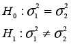
The test of hypotheses about two variances uses the F distribution. Recall that we discussed the F distribution in Chapter 5 as the ratio of two chi-square distributions. Since we also know from Chapter 5 that sample variances have a chi-square distribution, it follows that the ratio of two sample variances would have an F distribution.

Image7541.EPS (7.2)

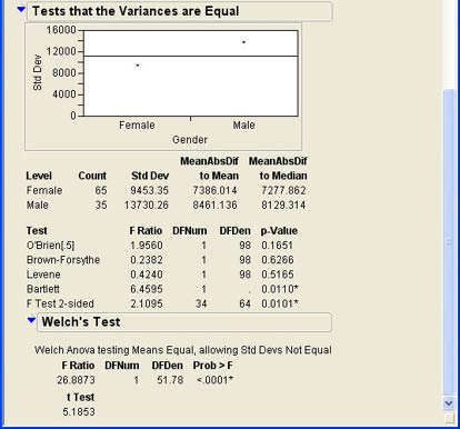
If the null hypothesis is true, the two sample variances should be about equal, and the ratio should be about 1.³ The test for two variances is accessed through the UnEqual Variances option shown in Figure 7.5. When Bob selects this option, the results shown in Figure 7.8 are appended to the results window. From the summary results, we can see that the standard deviation for the male salaries (13,730.26) is much larger than for females (9,453.35). However, this could be due to sampling error. The F test (F Test 2-sided) shows an F value of 2.1095 with 34 and 64 degrees of freedom. This value is the ratio of (13730.26)² divided by (9453.35)².The degrees of freedom are (n₁- 1) and (n₂- 1). The p-value is .0101, which is less than .05 so that we can reject the null hypothesis and conclude that the population variances are not equal. This means that we should not use the t-test for means that assume equal variances. It is a good idea to perform this test of the variances to make sure that the assumption of equal variances is reasonable. This test also tells us something important about the salaries at INCU.

Figure 7.8 Results of the Test of Two Variances

Equivalence Testing

Equivalence testing, which was introduced in the last chapter, is an option in JMP when there are only two groups.

Example 7.2

Ann Rigney recently had a discussion with Hank Wilson, the CFO at INCU, about the quality ratings. Hank expressed the opinion that male and female members valued different things in a credit union and that their impressions of quality were usually quite different. Ann found this argument less than convincing, and in analyzing the average responses to the overall quality question found no significant differences between males and females. However, she knew that accepting the null hypothesis would not impress Hank very much, so she decided to do an equivalence test of the differences. As in the last chapter, to perform an equivalence test, we need to specify a value (Δ) such that differences that are small or smaller would not be important differences in practice. Then we conduct two hypothesis tests:

Image4671044.EPS

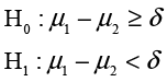
and

Image4673885.EPS

If we can reject both null hypotheses, we can say that the two groups are equivalent for our purposes. The problem is what to select for a value of Δ. From the descriptive analysis that Ann did earlier, she had noted that the standard deviation of the overall quality rating was 1.737. Ann figured that a difference of one half a standard deviation unit or less would be too small to be important. Since one half a standard deviation is .8685, she rounded off to .9 and decided to use this as the value of δ. Ann then loads the Customer Survey.jmp data table and selects Analyze → Fit Y by X from the JMP menu. She selects Overall as the Y, Column and Gender as the X, Factor and clicks OK. In the resulting drop-down menu () for the results, she selects Equivalence Test. When asked to enter a Difference considered practically zero, she enters .9 and clicks OK. The results window is shown in Figure 7.9

Figure 7.9 Results of the Equivalence Test

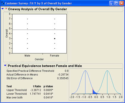
Since both tests have p-values less than .05, Ann concluded that there is no difference between the overall quality ratings of males and females.

Tests for Two Medians

The tests for two medians fall under what are often called nonparametric statistics. Nonparametric tests are sometimes called distribution-free tests because like the usual “parametric” tests they do not assume a normal distribution in the population. Discussion of these tests can be confusing because they are used for two different purposes.

As tests for whether two distributions are different when the usual assumptions of normality do not hold. If we assume that the distributions have the same shape and equal variances, this test can be used as a test for the equality of means when the population distributions are not normal.
As tests for location when scales are only ordinal (test of medians).

Our purpose here is to use the test for medians when scales are only ordinal. However, in JMP, the columns used for these test must be declared as continuous, not ordinal.

The nonparametric tests are accessed under the Nonparametric option as shown in Figure 7.10. As you can see, there are three different tests. The first is call the Wilcoxon test, which is based on the sum of the ranks in the two groups.

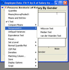
Figure 7.10 Nonparametric Options under Oneway

The second is the Median test, which is an extension of the sign test we discussed in Chapter 6.⁴ We will not discuss the van der Waerden test here. The null hypothesis for testing medians is

H₀: η₁= η₂

H₀: η₁≠ η₂

Example 7.3

Ann Rigney, VP of Marketing, believes that some of those who rated quality lower in the survey were members who did not take advantage of all of the services offered by INCU. One way to test this is to see if there are differences in the overall quality rating between those who use certain services and those who do not. She decides first to look at the impact of ATM use on quality ratings. Since she still is concerned that the quality ratings may only be an ordinal scale, she decides to perform nonparametric tests.

Opening up the customer survey.jmp data table, Ann selects Analyze → Fit Y by X from the JMP menu. In the dialog, she selects Overall as the Y, Column and ATM as the X, Factor. After she clicks OK, she observes the results shown in Figure 7.11.

Figure 7.11 Initial Results for Example 7.3

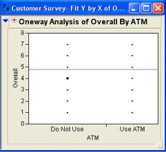
It is not immediately obvious to Ann whether there is a difference between the two groups or not. She decides to perform both a Wilcoxon test and a Median test to see if there are significant differences between those who use the ATM machines and those who do not.

Ann clicks the drop-down menu () next to the One Way Analysis of Overall by ATM in the report to access the options menu and selects Wilcoxon Test from the menu. Repeating this and selecting Median Test, she obtains the two additions to her results window shown in Figure 7.12.

Figure 7.12 Nonparametric Results for Example 7.3

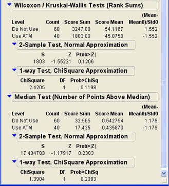
The Wilcoxon test first rank orders all of the observations without regard to which group they are in and then sums the rank value for each group. These are the Score Sum values shown in Figure 7.12. The S test statistic shown in the 2-Sample Test Normal Approximation section is the minimum of these values. JMP uses the normal approximation to the Wilcoxon distribution to calculate a p-value. In this case, the p-value is .1206, which is not significant. Ann cannot conclude that ATM use influences the overall quality rating. JMP also displays a chi-square approximation test, which shows much the same results.

The Median test results are displayed in the next section of Figure 7.12. As we found with the Wilcoxon test, we cannot reject the null hypothesis of equal medians with the Median test since the p-value is .2383. Notice that the p-value for the Median test is larger than the p-value for the Wilcoxon test. This is usually the case. The Wilcoxon test is generally more powerful than the Median test. This has led some to conclude that the Median test is obsolete and should not be used anymore.⁵ However, the Wilcoxon test assumes that the two population distributions have the same shape and the same variance. If this is not true, then one must use the Median test.

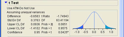
Ann notices that the p-value for the Wilcoxon test is not extremely high and wonders what would happen if she assumed that the rating scale was an interval scale and performed a normal t-test on the data. Going back to the drop-down menu, she selects the t Test option to perform an unequal variance t-test on the data. The results are shown in Figure 7.13. Ann notes that the p-value of .0851 is smaller than it was with the nonparametric tests but still not significant. Ann knows that the p-value should be smaller since nonparametric tests are not as powerful as their parametric counterparts. Ann is forced to conclude that ATM use likely has little impact on quality ratings.

Figure 7.13 Unequal Variance t-Test for Example 7.3

Dependent Groups

So far we have assumed that the groups are independent. When it comes to variables like gender and ATM use, this makes sense. There is no relationship between the two groups. We will now turn to a situation where dependent samples make sense and discover how to analyze such situations in JMP.

Example 7.4

Mary Warner, the COO at INCU, has decided to conduct some experiments to see if there are ways to shorten the waiting lines at the branch locations of INCU. Right now, the teller windows at the branches are set up so that each teller has her own waiting line and arriving customers can go to any teller that they wish. Mary has read that this kind of arrangement is not as efficient as a single queue with ropes so that arriving customers stand in a single line and take the next available teller. Mary knows that some customers may not like this arrangement, especially if they have a favorite teller that they normally go to. Because of this concern, she wants to make certain that this kind of arrangement is more efficient before committing to the change. She decides to experiment with the two arrangements in a sample of branch locations. She will have student interns at the credit union observe the lines and record the time that each customer waits in line during certain times of the day. Branches in one group will maintain the current configuration, and branches in the other group will change to the new, single waiting line arrangement. The average wait times for the two configurations will help Mary decide.

Mary knows that she should assign the selected branches randomly to the two groups, but she also knows that the wait times at branches are heavily influenced by traffic volumes, which differ from one branch to another. Therefore, she decides to carefully match branch banks in the new configuration with branches of similar traffic volumes with the old configuration. In this way, these differences in traffic volumes are balanced between the two groups. However, the groups are now no longer independent.

Dependent groups in JMP are analyzed using the Matched Pairs platform. This platform requires that the data be in a different format. To use this platform, the observations for each group must be in separate columns rather than in a single column with the grouping indicated by a second column. Further, each observation in the matched pairs must be in the same row.

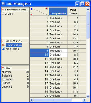
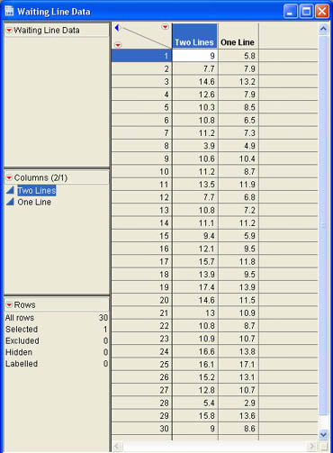
Unfortunately, Jim Plummer, who was assigned to collate the data and put it into a JMP data table, was not aware of this. When Mary received the initial data from Jim (Initial Waiting Data.jmp), she noticed that it was in the wrong format (see Figure 7.14). Mary sent the data table back to Jim with a note explaining that she needed the waiting time data in separate columns. When Jim received the e-mail from Mary, he knew that he could quickly fix the data table using the Table → Split command in JMP. The Split command (and its inverse Stack command) allows you to split a column into two columns based on a second column (stack two separate columns into a single column). Jim selects Table → Split from the JMP menu to show the dialog illustrated in Figure 7.15. Jim first selects the Wait Times column and clicks Split Columns to indicate to JMP that he wants to split the data in that column into two columns. He then selects the Configuration column and clicks Split By to indicate that the column is to be split based on the values in this column. Jim also has options on what to do with other columns in the data table under the Remaining Columns heading, which allow him to keep all of the columns, drop them all, or select which columns are retained in the new data table. Since there are no other columns, Jim ignores this section.

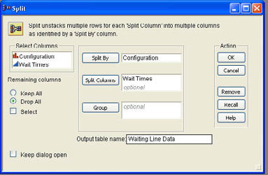
Figure 7.14 Initial Waiting Line Data Table

Figure 7.15 Split Column Dialog

There is also a place (Output table name) to enter a name for the new data table. Joe enters Waiting Line Data in this box and clicks OK to create the new data table, which is shown in Figure 7.16.

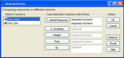
Figure 7.16 Split Data Table for Waiting Line Data

After Mary receives the revised data table back from Jim, she selects Analyze → Matched Pairs from the JMP menu to perform the analysis. The Matched Pairs dialog is shown in Figure 7.17. Mary selects both columns, clicks on Y, Paired Response, and then clicks OK. The results window for the analysis is shown in
Figure 7.18.

Figure 7.17 Matched Pairs Dialog

Figure 7.18 Results Window for Matched Pairs Analysis

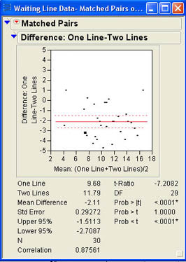
The matched pairs t-test is performed on difference scores. In other words, JMP takes the difference between each time in the two-line configuration, subtracts the time in the one-line configuration, and then does a regular t-test on these difference scores (the same t-test we discussed in Chapter 6). Mary sees that the average time difference between the two configurations is 2.11 minutes and that the difference is highly significant with a p-value of .0001 or less.

You might be wondering why it makes a difference how we analyze this data. What would happen if Mary had not recognized the difference between dependent samples and independent samples and analyzed the original data as she received it from Jim? Figure 7.19 shows the results of using the original data, the Fit Y by X platform, and selecting Means/Anova/Pooled t from the Oneway options to analyze the data. We can see that the t ratio is 2.55 with a p-value of .0135. Compare this with the results of the matched pairs analysis, where the t value was 7.2082 and the p-value was less than .0001.

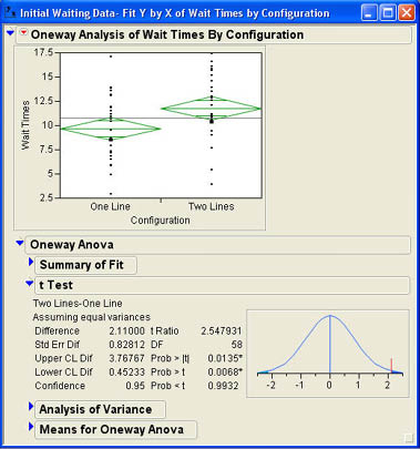
Figure 7.19 Analysis of Waiting Times Using Independent Groups Test

Although both results indicate a significant difference in waiting times, the t value for the matched pairs design is much larger and the p-value is smaller by a factor of more than 100. Examining the results closely we see that the average difference is 2.11. This is the same value as the average of the difference scores. Since the t ratio is the ratio of the sample difference (the same in both analyses) divided by the standard error, the difference in results has to be in the standard error term. Looking at Figure 7.18, we can see that the standard error for the matched pairs design is .29272, while Figure 7.19 shows a standard error of .82812, almost 4 times as large. This is the power of dependent samples; removing the variability due to the matching factor (in this case traffic volume), yields a much more powerful test of the differences being tested.

Qualitative Variables with Three or More Levels

So far we have restricted our discussion to qualitative variables with only two levels. We now want to turn to situations where the qualitative X factor has three or more levels. We will again look at means, variances (standard deviations) and medians. Although some of the terminology may seem somewhat different, the tests that we discuss here are in many ways just extensions of the pooled tests that we discussed for two groups.

Tests for Three or More Means

With three or more groups, the general null hypothesis is

H₀: µ₁ = µ₂ = µ₃ = . . . . . = µ_a

H_A: not (µ₁ = µ₂ = µ₃ = . . . . . = µ_a)

where a is the number of groups or levels of the qualitative factor. It is important to note that the alternative hypothesis does not say that all the means are different. It simply says that they are not all the same. This means that at least two of them must be different. This is easiest to see with three levels of the qualitative factor so that we have three groups. The hypotheses would then be

H₀: µ₁ = µ₂ = µ₃

H_A: not (µ₁ = µ₂ = µ₃)

If the null hypothesis is false, there are four possibilities for the alternative hypothesis:

µ₁ = µ₂ ≠ µ₃ µ₁ ≠ µ₂ = µ₃ µ₁ = µ₃ ≠ µ₂ µ₁ ≠ µ₂ ≠ µ₃

In only one of these cases, are all four means different. This has some important consequences as we will see later.

In addition to the null and alternative hypotheses, we also need to make some additional assumptions before proceeding:

Normality: The populations follow a normal distribution within each group.
Homogeneity of variances: The population variances are the same in each group
Independence: Experimental units are assigned randomly to each group so that the groups are independent.

Note the similarity between these assumptions and the pooled independent group t-test we discussed above. In fact, as we will see, ANOVA is an extension of the pooled two-group t-test.

The general technique for analyzing the impact of a qualitative variable with three or more levels on a quantitative variable is analysis of variance (ANOVA). At first it may seem confusing that we are testing a hypothesis about means by analyzing variances. To understand the logic of ANOVA, we need to understand the concept of partitioning variability. It is easiest to illustrate that in the context of an example.

Example 7.5

Mary Warner and Ann Rigney were discussing member perceptions of quality, and Mary began to wonder what role the physical facilities and employee attitudes might play in quality perceptions. Going over the design of the customer survey, she noticed that there were no variables that indicated which branch each customer used for most of their transactions. However, it was well known that most members used branches near where they lived, so she thought that the zip code information might serve as a reasonable proxy for the branch that the member used.

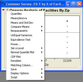
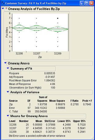
Mary asked Angie Nelson, Customer Experience Manager, to look at the data to see if she could find anything that they should look at more closely. Angie decided to look at the impact of zip code on both the perceptions about the facilities (Facilities) and the attitudes of the employees (Attitudes). First examining the Facilities column, Angie selects Analyze → Fit Y by X from the menu and selects Facilities as the Y, Column and Zip as the X, Factor. The results along with the Oneway menu are shown in Figure 7.20. Notice that the options menu is somewhat different for three levels of the qualitative variable as opposed to two levels. Since she is testing means, Angie selects the Means/Anova option. The results window then changes to that shown in Figure 7.21. The results window for analysis of variance consists of three sections in addition to the graph with mean diamond plots: Summary of Fit, Analysis of Variance, and Means for Oneway Anova. The summary of the means in the last section shows that the three means are very nearly equal, which is reflected in the means diamond plots. The central portion of the output is the ANOVA table shown in the Analysis of Variance section.

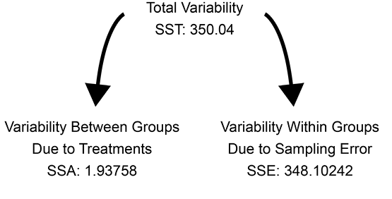
Figure 7.20 Results for Example 7.5 with Oneway Menu

The ANOVA table lists the sources of variability (Source), the degrees of freedom (DF), the sum-of-squares for each source (Sum of Squares), the mean square for two of the sources (Mean Squares), an F value (F Ratio), and a p-value (Prob > F). There are three sources of variability in the first column of the table: the total variability of all of the values (C. Total); the variability between groups, which is due to the treatment or grouping variable (in this case Zip); and within-group variability, which is a reflection of sampling error (Error). It is the sum-of-squares that reflect the breakdown of variability into parts. Figure 7.22 shows the basic concept. The total variability of all of the data (350.04 in Figure 7.21) is broken down into two parts. The first is the variability between groups, which reflects the impact of the treatment variable (1.93758 in Figure 7.21). The second part is the variability within groups, which reflects sampling error (348.10242 in Figure 7.21). The breakdown of the total variability into component parts is at the heart of analysis of variance, and is also very important in regression analysis as we will see in Chapter 9.

The logic of ANOVA is that variability within each group should just represent sampling error due to taking a random sample for each group. If the null hypothesis is correct—i.e., all the means are equal—variability between the groups should also just be reflective of sampling error. However, if the null hypothesis is wrong and the population means are not the same, then variability between the groups should be greater than would be expected from sampling error and should be greater than the variability within groups.

Figure 7.21 Oneway ANOVA Results for Facilities

Figure 7.22 Breaking Down Total Variability

To test this hypothesis, we divide the sum of squares by the degrees of freedom to obtain what is called a mean square. A mean square is simply a variance. If the null hypothesis is true, both variances (within groups and between groups) should be the same. As we saw earlier in this chapter, to test for the equality of two variances, we use an F ratio as shown in Figure 7.21. It is in this way that we use variances to test a hypothesis about means.

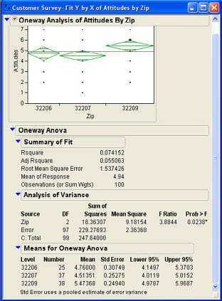
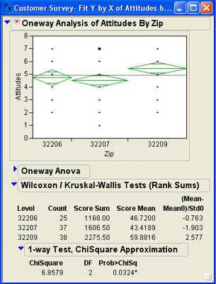
Angie can see from the ANOVA results that there is no difference in quality perceptions between the three zip codes. She conducts the same test for the Attitudes column and observes the results in Figure 7.23. Here Angie notes that the F test is statistically significant with a p-value of .0238. This tells her that the customer responses to the Attitudes question were not the same in all the zip codes.

Figure 7.23 Oneway ANOVA Results for Attitudes

Comparison of Means

In the test for Attitudes, we saw that Angie can reject the null hypothesis. This tells her that not all of the means are equal. But remember, it does not tell us that all of the means are different, nor does it tell us where the differences are. To find out which means are significantly different, we must do what are called multiple comparison tests.⁶ To compare the means after a significant F value in the analysis of variance, use the Compare Means option as shown in Figure 7.24. There are a wide variety of multiple comparison tests in the literature. JMP offers four options here. The fourth option, With Control, Dunnett’s, is a specialized option used only when one of the levels of the X, Factor is a control group. We will not discuss this option here.

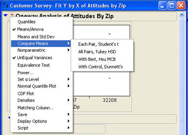
Figure 7.24 Compare Means Option in Oneway

The first option, Each Pair, Student’s t, performs a Student’s t-test for each pair of means. This method is not generally recommended because it does not control for the overall risk of a Type I error. The third option, With Best, Hsu MCB, is most useful for situations where there are a large number of levels of the X, Factor, and we are interested in finding the best value.

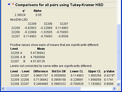
The one most widely used is the second option, All Pairs, Tukey HSD. Although this test is more conservative than the first option of separate Student’s t-tests, it does control the overall Type I error rate and is therefore to be preferred. The results of this option for the Attitudes analysis are shown in Figure 7.25. As you can see, the only statistically significant difference is between zip codes 32209 and 32207. Therefore, we can say that the quality ratings for employee attitudes were definitely better in zip code 32209 than they were in zip code 32207. We may want to look at the differences in management and employees at the different branches in these zip codes to see if there are positive (or negative) aspects of these situations so that we can use this knowledge to improve quality perceptions at the other branches.

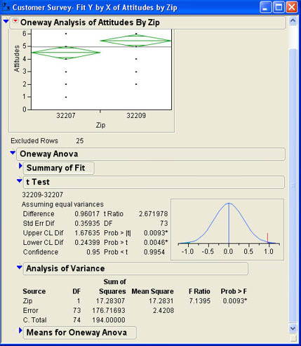
Figure 7.25 Results of the Comparison of Means for Attitudes

ANOVA and the t-test for Two Groups

At the beginning of this section, we alluded to the similarities between the oneway analysis of variance and the pooled variance t-test for two groups. To explore this connection, we will reanalyze the data on Attitudes with one of the zip codes (32206) excluded from the analysis leaving only two groups. The results are shown in Figure 7.26. Notice that the p-value for the two-tailed t-test is exactly the same as the p-value for the F test in the ANOVA table. Also notice that the F Ratio in the ANOVA table (7.1395) is the square of the t Ratio in the two-group t-test (2.671978). This implies that the two analyses are entirely equivalent. For two groups, the ANOVA F test and the two-group t-test are the same. It is in this sense that analysis of variance is an extension of the two-group pooled variance t-test to three or more groups.

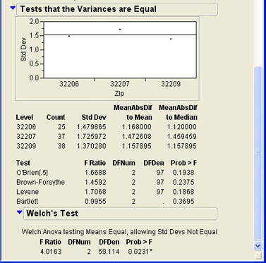
Figure 7.26 Comparison of Oneway ANOVA and Two Group t-test

Tests for Three of More Variances

As with the t-test for two means, we may want to test the assumption of the equality of the variances—i.e., the homogeneity of variances assumption that underlies ANOVA. As with testing two variances, the tests for three or more variances are located under the drop-down menu at the top of the report under the Unequal Variances option. When Angie selects this option with the analysis for Attitudes, the results shown in Figure 7.27 are added to the results window. Note that there are four tests shown to test the equality of the variances. The F Ratio that we used for two groups is no longer shown because we have more than two groups. The Bartlett test is generally not recommended because it is quite sensitive to the violations of normality assumption. The other three tests usually give very similar results. In this case, although the standard deviation in the 32207 zip code is slightly higher than in the other two, the results are not statistically significant.

Figure 7.27 Results of the Unequal Variance Option for Attitudes

Tests for Three or More Medians

The tests for three or more medians are accessed in exactly the same way as for two medians that we discussed earlier. Again, these tests are accessed under the Nonparametric option in the Oneway results window. Angie is somewhat concerned that the scales used for the Facilities and Attitudes columns may only be an ordinal scale. To make sure that the results for the Attitudes column still holds for ordinal scales and medians, she decides to perform a nonparametric analysis of this column. She selects the Wilcoxon option, which produces the results shown in Figure 7.28.⁷ These results very closely mirror those for the parametric analysis above.

Figure 7.28 Nonparametric Results for Attitudes

Summary

This chapter explores the impact of a qualitative variable on a quantitative variable. A qualitative variable divides the data into groups or levels. Tests for two groups or levels are discussed first. An important distinction is between independent and dependent groups. Dependent groups occur when the elements of the groups are related in some way. They may be the same elements in both groups as in before-after tests, or the elements in the groups may be matched on the basis of some characteristic. Most of the tests described in this chapter utilize the Fit Y by X platform of JMP. There are two different tests for independent group means. One assumes that the population variances are equal and pools the separate sample variances in calculating the standard error. The other test does not assume equal variances and calculates the standard error based on the separate sample variances. The F test to test the equal variance assumption is also described in this chapter. Equivalence testing can be used to provide support for the proposition that the difference between two group means is small enough to be essentially zero. The Wilcoxon Rank Sum test and the Median test can be used to test hypotheses about two population medians.

The Matched Pairs platform can be used to test for the equality of means in two dependent groups. The advantage of dependent groups is that it provides a more powerful test of the difference between the means in most situations.

Tests where the qualitative variable has three or more levels are all performed with the Fit Y by X platform. Tests for means are conducted using analysis of variance (ANOVA), which tests a hypothesis about means by testing the ratio of two variances. The technique divides the total variability of the observations into between-group variability and within-group variability. If the group means are equal in the population, then both within-group variability and between-group variability are estimates of the same population value. If the null hypothesis is false and the population means are not equal, then between-group variability should be larger than within-group variability, and the F ratio tests for the equality of these two variance components. A significant F ratio can be followed by multiple comparison tests to determine which specific means are different from one another. A demonstration is provided that shows that for two groups, the ANOVA is equivalent to the pooled variance t-tests for two means.

Tests for the equality of three or more group variances and three or more medians can also be performed using the Fit Y by X platform.

Chapter Glossary

analysis of variance (ANOVA: A technique that tests for the equality of means by partitioning the variability in the data and looking at the ratio of the two variance components.
correlated: Two things are correlated when they are related in some way.
homogeneity of variances: An assumption that the variances of all groups being tested are equal in the population.
levels: The number of values taken on by a qualitative variable. Equivalent to the number of groups in the analysis.
mean square: The sum of squares divided y by the degrees of freedom, which is another term for a variance.
multiple comparison: A simultaneous comparison of a set of means looking for significant differences performed after a significant F test in ANOVA.
nonparametric statistics: Statistical tests that do not assume that the populations involved have a normal distribution and that can be used for ordinal scale variables.
statistically significant: The null hypothesis can be rejected.

Questions and Problems

Hank Wilson the CFO of INCU is curious about differences between those members who take out loans from INCU versus those that do not. In particular, he wonders if there is a difference in age or tenure with the bank in these two different groups.

1. Conduct the relevant analyses for Hank. What can you tell him about differences between those who have loans with INCU and those that do not?

Darrel Young, the CTO at INCU, is becoming increasingly aware of the cost of PCs at INCU with the increased pressure to reduce costs during the current recession. Darrel wonders if the data gathered on PCs in Chapter 2 (Computer Info Final.jmp) can tell him anything that might help him reduce costs for PCs. Two questions in particular occur to him.

2. Is there a difference between PCs, Macs, and Linux computers? Conduct the appropriate analysis. What can you tell Darrel about the costs of the machines?

3. When there are multiple vendors for the same type of machine (as there are with PCs), is there a cost difference between the vendors? Which vendor would you recommend based on your analysis?

Alice Hansen has been working on planning manpower resources for the future at INCU. There are several issues that she is considering that the employee data (Employee Data.jmp) may help answer.

4. Are there significant differences between male and female employees at the bank in terms of age? You should evaluate differences in the mean, standard deviation, or median age.

5. Because of concerns over when people will retire and leave the credit union, Alice is also concerned about differences between males and females in terms of their seniority at the bank. What can you tell her about any such differences?

6. Alice also would like to know if there are departmental differences in terms of the age of the employees. In other words, are there particular areas or departments where the employees are older and more likely to be retiring soon?

Bob Reed, who works for Alice Hansen in HR, recently read an article that stated that lower income employees were bailing out of company health plans because of the high costs and signing up for state discount health plans instead.

7. As a surrogate, Bob wonders if there are differences in the mean or median salaries of those who are enrolled in the company health plan versus those who are not. What can you tell Bob about this based on the sample data?

8. Bob is also concerned that the company may be left primarily with older workers, whose health costs tend to be higher, enrolled in their health plan. Based on the ages in the sample data should Bob be concerned about this?

References

Freidlin, Boris, and Joseph L. Gastwirth. 2000. Should the Median Test Be Retired from General Use? The American Statistician 54, 3, 161-164.

Notes

1 Note that this is different from tests for means using the normal or t distribution where the Z or t value should be about 0 under the null hypothesis.

2 This form is the genesis of the term null hypothesis in that the null hypothesis states that the difference is null or zero.

3 Note that this is different from tests for means using the normal or t distribution where the Z or t value should be about 0 under the null hypothesis.

4 To further confuse matters, the Wilcoxon test is entirely equivalent to the Mann-Whitney U test and is sometimes called the Mann-Whitney-Wilcoxon test. The Median test is also sometimes called the Mood Median test and even the Brown-Mood Median test.

5 For example, see Freidlin and Gastwirth (2000).

6 Since these tests are done only after finding a significant F value in the overall ANOVA test, these tests are sometimes also called post-hoc tests.

7 Note that the test for three or more medians is more properly called the Kruskal-Wallis test. This is why the results are labeled Wilcoxon/Kruskal-Wallis Tests.

..................Content has been hidden....................

You can't read the all page of ebook, please click here login for view all page.

Table of Contents for Part 4 The Effects of One Variable on Another

Create new playlist

Sign In

Sign Up

P a r t 4

The Effects of One Variable on Another

Chapter 7 Effects of a Qualitative Variable on a Quantitative Variable

Chapter 8 Effects of a Qualitative Variable on a Qualitative Variable

Chapter 9 Effects of a Quantitative Variable on a Quantitative Variable

Chapter 10 Effects of a Quantitative Variable on a Qualitative Variable

C h a p t e r 7

Effects of a Qualitative Variable on a Quantitative Variable