
Binomial Regression and the Logic of Logistic Regression
Multinomial Logistic Regression and ANOVA
In this chapter, we will briefly introduce you to the fourth, and final, component within the Fit Y by X platform. This platform, called the Logistic platform, examines the effect of a quantitative variable on a qualitative variable, either nominal or ordinal. In concept, it is similar to our discussion of regression in Chapter 9, and, in fact, is often called logistic regression. From a mathematical point of view, however, the regression analysis discussed in this chapter is very different from the linear regression discussed in Chapter 9. Since the Response is a qualitative variable rather than quantitative, our goal is to predict the group in which an observation will fall rather than a precise value. Also, since the assumption of a normal distribution no longer applies, the fitting function is much different than in Chapter 9.
The simplest case is when the Response variable has only two possible values. This is called binomial regression. The more general case with multiple values of the Response variables is called multinomial regression. We will first explore the logic of logistic regression in the context of binomial regression and then expand that to illustrate multinomial regression.
The Situation at INCU
Ann Rigney has been going over the survey of potential customers with Jack Snowden and Betty Anderson. Ann is intrigued by the implications of some of the data and feels that from a marketing point of view, they may be able to use the data to try to identify which potential customers would be most beneficial to pursue as possible new members at INCU. In particular, she would like to identify which types of customers were most likely to be unhappy with their current financial institution and therefore most open to changing banks. She asks Jack and Betty to see if they can use either age or the amount of deposits to predict whether or not a customer is happy with their financial institution.
Binomial Regression and the Logic of Logistic Regression
In binomial regression, the Response column has only two values, one of which we can call a success and the other a failure. The name obviously comes from the Binomial distribution first discussed in Chapter 5. The purpose of binomial regression is to predict whether something will be a success or a failure. More precisely, the goal of binomial regression is to predict the probability that the response Y is a success rather than a failure. This is similar in concept to our discussions of proportion of successes in previous chapters. The term logistic regression comes from the logistic curve that is fit to this model rather than a straight line as in linear regression. Figure 10.1 shows the difference between the two curves being fitted.
Figure 10.1 Logistic Regression Curve Contrasted with Linear Regression
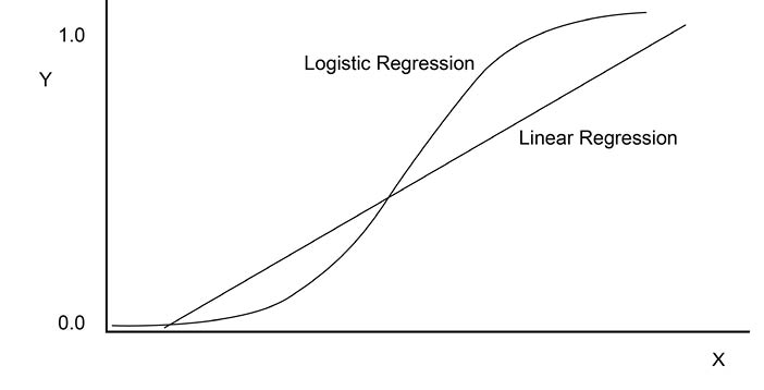
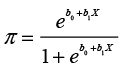
Since we are trying to predict a probability (proportion) that must be between 0 and 1, the logistic curve is better than the linear curve because it is by definition restricted to the area between 0 and 1 while the linear curve is not. Also, most of the curve is near 0 or 1, which are the values of our dependent variable (Response). The equation for the curve is rather complex. Let π be the probability of a success. Then the equation for π is
 (10.1)
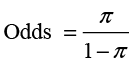
where e is the base of the natural logarithms. The logistic curve is decidedly nonlinear, but we can make the equation linear by converting to odds and taking the logarithm. Odds are defined from probabilities as
 (10.2)
Then
 (10.3)
where ln is the natural logarithm. The left side of the equation is called a log odds or logit for short. In practice, logistic regression attempts to fit Equation 10.3 to the data. An additional complication is that there is no closed-form equation to solve for the values of b0 and b1 as there is in linear regression. Rather, the solution procedure must proceed by iterating from one solution to another.
Another difference between logistic regression and linear regression is that logistic regression uses a maximum likelihood approach to derive the fitted equation rather than the principle of least squares used in ordinary regression. Although the basic concept of predicting a Response value from a Factor is the same in logistic regression as in linear regression, the details of the process are quite different.
The Logistic Platform
As with most of the analysis we have done in the previous three chapters, logistic regression starts from the Fit Y by X platform. However in this situation the Factor or predictor variable is a continuous variable and the Response is a qualitative variable.
Logistic Regression
We will illustrate the basics of logistic regression with an example.
Example 10.1
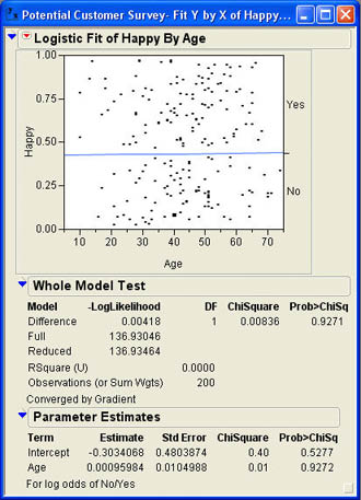
Jack and Betty decide to begin by trying to first predict a customer’s happiness with their financial institution from age. Jack loads the data table Potential Customers.jmp and selects Analyze → Fit Y by X from the JMP menu. In the dialog, he selects Happy as the Y, Response and Age as the X, Factor. After he clicks OK, the results window opens with the plot shown in Figure 10.2.
The results window first shows a logistic probability plot. The plot shows the probability of a No or a Yes response as a function of Age. Since the slope of this line is essentially zero, that tells us that the probability of a No response does not change as Age changes. This is our first indication that Age does not help in predicting whether or not a person will be happy with their financial institution.
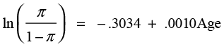
The parameters of the model are shown in the section Parameter Estimates. The estimate of the intercept (b0) is -.3034, and the estimate of the slope (b1) is .0010. The parameter estimates must be interpreted within the context of Equations 10.1 and 10.3. Before using the equations, we need to know how the odds ratio was formed (i.e. which probability appears in the numerator and which is in the denominator). At the bottom of the results section is the statement For log odds of No/Yes. This means that the odds are referring to the odds of a No response to the question of whether or not they were happy with their financial institution. In other words, the odds are for an unhappy response. Using Equation 10.3, we would have
As in regression, rarely are we interested in the intercept term, but the slope can be interpreted in terms of the odds ratio. The .001 value means that for each additional year of age, the odds that the response will be No go up by .001. If we want to use the parameters to make a prediction, we must use Equation 10.1. For example, the probability that a member 40 years old will respond No is
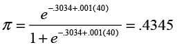
Figure 10.2 Logistic Results for Age Predicting Happiness
A significance test is also shown for each parameter. Rather than a t ratio for each estimate, a chi-square statistic is given. This test statistic is sometimes called the Wald test. The chi-square value is calculated as
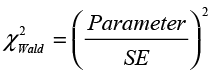 (10.4)
where parameter is the value of the parameter estimate and SE is the standard error. As can be seen in Figure 10.2, neither parameter is statistically significant. The fact that the slope is not significant was hinted at in the scatter plot where the best fitting line is virtually flat.
As with regression analysis, there is a test of the overall fit for the model as well as tests for the individual parameters. The results for the model tests are contained in the Whole Model Test section of the results. The column headed Model lists Difference, Full, and Reduced. These stand for the full model, the reduced model, and the difference between them. The full model is the model estimated by the procedure. The reduced model uses only the marginal probabilities from the data for prediction. Since 87 out of the 200 responses are No, the marginal probability of a No response is 87/200 = .435. Therefore, the predictions for the reduced model would be .435 for a No response and .565 for a Yes response for any age.
The column labeled –LogLikelihood contains the value for the negative log of the likelihoods for the full and reduced models and the difference between them. The log likelihood is a measure of uncertainty where a larger value indicates better fit. What is important is the difference between the log likelihood for the full model and the log likelihood for the reduced model. This difference is the increase in fit from using the model over using the marginal probabilities. Figure 10.2 shows that this difference is very small.
The chi-square distribution is used to test the significance of the increase fit from the model. Two times this difference has a chi-square distribution with degrees of freedom equal to the number of values for the Response column minus 1—in this case, 2-1 = 1 degree of freedom. The p-value of .9271 tells us that the overall model is not statistically significant. In other words, using age as a predictor does not give us any better predictions of the happiness response than simply using the marginal probabilities.
Example 10.2
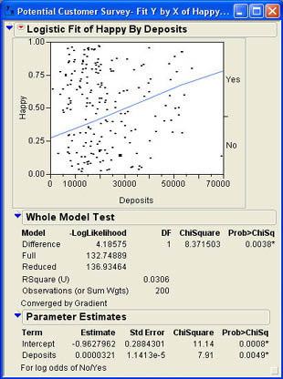
Betty and Jack next decide to try Deposits as a predictor of happiness. Repeating the process but this time selecting Deposits as the X, Factor produces the results shown in Figure 10.3. The scatter plot immediately tells us that Deposits are a better predictor of happiness than Age was since the slope of the best fitting line is definitely nonzero. The test of the whole model produces a larger difference in the log likelihood values and a p-value of .0038 indicating that the model significantly improves the predictions over the reduced model.i
The parameter estimates are b0 = -.963 and b1= .0000321. The resulting prediction equation for odds is
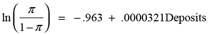
The slope is a small value because of the magnitude of the numbers involved in deposits. The .0000321 indicates that each additional dollar in deposits increases the odds that the individual will be unhappy by .0000321. In this situation, it makes more sense to translate the statement into thousands of dollars, which is more representative of the values in the data. Then the slope would state that for each additional thousand dollars in deposits the odds of an unhappy response go up by .0321.
Figure 10.3 Logistic Results Using Deposits as the X Factor
It is easier to see the value in the model when predicting probabilities. Recall that 43.5% of the responses in the sample were No responses. That means that without knowing anything, our best estimate for the probability of a No response would be .435, its marginal probability. Suppose that we know that the individual in question has deposits of $50,000. Then using the model, our predicted probability of a No response would be
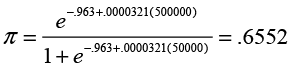
Knowing the amount of the deposit changes our estimate of the probability by a considerable amount over the marginal probability.
We can also see in Figure 10.3 that both the intercept and the slope are significantly different from zero with p-values of .0008 and .0049 respectively.
Inverse Prediction
Our goal in prediction with logistic regression is to predict a probability of occurrence for a value of the Response for a given value of the Factor. Inverse prediction then is to predict the value of the Factor, given a probability for a value of the Response. This is similar to the situation of finding percentiles in probability distributions in Chapter 5.
For example, we might want to know the deposit level such that there is a 50/50 chance that the individual will be unhappy with their financial institution. Deposit levels below this would lead the individual to be happy with their institution and levels above this would lead the individual to be unhappy. We could use the crosshairs tool on the logistic probability plot to find the value where .5 intersects with the logistic curve, but that is rather imprecise.1 We can use the Inverse Prediction option that is accessed by selecting the drop-down menu (![]() ). The available options for the Logistics analysis are shown in Figure 10.4.
). The available options for the Logistics analysis are shown in Figure 10.4.
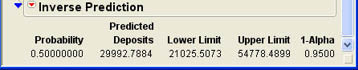
When the Inverse Prediction option is selected, the results window will expand and the dialog shown in Figure 10.5 will be added to the bottom of the window. Enter one or more probabilities in the indicated boxes and then click Run. In Figure 10.5, the .5 probability has been entered. When you click Run, the results window changes, and the Inverse Prediction section looks like that shown in Figure 10.6. The results indicate that the 50/50 dividing line is very close to $30,000 ($29,992.79 to be exact). Depositors with more than $30,000 in deposits are more likely to respond No, while those with less than $30,000 will be more likely to respond Yes. JMP also provides a 95% confidence interval for this inverse prediction.
Figure 10.4 Logistic Options Menu
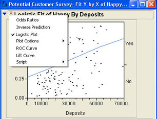
Figure 10.5 Inverse Prediction Dialog
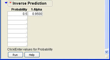
Figure 10.6 Inverse Prediction Results for a Probability of .5
Multinomial Regression
The basics of logistic regression just discussed for binary Response variables can be extended to Response variables with multiple levels. The graphs can get harder to follow with multiple levels of the Response, but the basic principles are the same.
A Multinomial Example
To get a feel for multinomial regression we will return to the situation at INCU.
Example 10.3
Jack and Betty decide to explore the data a little more to get a better feel for logistic regression. They decide to try to predict which institution a member belongs to based on the amount of their deposits. Using Deposits as the X, Factor and Institution as the Y, Response, they obtain the results shown in Figure 10.7. The Whole Model Test result indicates that the model is highly statistical significant with a p-value of .0001. The RSquare value is .3714, which is quite high for predicting a nominal variable. The difficulty comes in interpreting the graph, which is much more complex than for the binomial regression. Remember that logistic regression is predicting an odds ratio that is a ratio of two probabilities. Logistic regression uses one group as the reference point (denominator) for all of the odds ratios. In this case, the reference group is Keystone.2 Each odds ratio then uses the probability of Keystone as the denominator.
The bottom curve represents Wash Interstate, the second curve represents North Idaho, the third State Employee, and the fourth curve represents Meta Credit. The probabilities where the points meet the Y axis are cumulative probabilities. Individual probabilities for each category of the Response are represented by the space between the curves. The probability of the individual being a member of Wash Interstate for any value of Deposits is the distance of the first curve from the X axis. The probability that the individual is a member of North Idaho is the distance between the first curve and the second curve, and so on. The probability of the last category, the reference group Keystone, is the distance between the last curve and the top of the chart.
Figure 10.7 Logistic Results for Deposits Predicting Institution
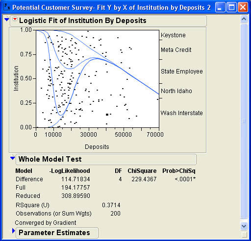
To help in understanding the chart, several vertical reference lines (the straight lines) have been superimposed over the chart produced by JMP. These lines are not part of the normal output. The first reference line is located at a little less than $10,000. At this point, the first curve is still on zero, which indicates that an individual with this level of deposits ($10,000) has virtually no chance of being a member of Wash Interstate. The distance from this curve and the curve line is about .60 indicating that there is about a 60% chance of an individual with $10,000 in deposits being a member of North Idaho. The distance from the second to the third curve is about .26 indicating that there is a 26% chance that an individual with $10,000 in deposits is a member of State Employee, and the distance between the third curve and the fourth curve is about .14 indicating a 14% chance that an individual with $10,000 in deposits is a member of Meta Credit. Since the fourth curve is at the top of the chart, the chance that an individual with $10,000 in deposits is a member of Keystone is virtually zero. Notice that the probabilities have to add up to 1.0.
The second reference line is placed at about $16,000. The height of the first curve at this point is about .15 indicating a 15% chance that an individual with this level of deposits is a member of Wash Interstate. The distance between the first and second curves is zero (the lines have merged) indicating a 0% chance of the individual being a member of North Idaho. The third curve is at about .60 for this level of deposits, so the distance between the second and third curves is .60 - .15 = .45 indicating a 45% chance the individual is a member of State Employee. The fourth curve is at about .98, which means a 98 - .60 = .38 or 38% chance of the individual being a member of Meta Credit. This means that there is a 2% chance (1.0 - .98) of the individual being a member of Keystone. Again, the probabilities add up to 1.0.
The third vertical reference line at a little less than $30,000 indicates the following probabilities: Wash Interstate .65, North Idaho .00, State Employee .05, Meta Credit .15, and Keystone .15.
The fourth vertical reference line is drawn at $50,000 and indicates about a 59% chance that the individual is a member of Wash Interstate, a 41% chance they are a member of Keystone, and a 0% chance for the other institutions. The results for the four scenarios are summarized in Table 10.1
Table 10.1 Summary of the Scenario Probabilities
| Scenario 1 | Scenario 2 | Scenario 3 | Scenario 4 | |
|---|---|---|---|---|
| About 10,000 | About 16,000 | About 30,000 | About 50,000 | |
| Wash Interstate | .00 | .15 | .65 | .59 |
| North Idaho | .60 | .00 | .00 | .00 |
| State Employee | .26 | .45 | .05 | .00 |
| Meta Credit | .14 | .38 | .15 | .00 |
| Keystone | .00 | .02 | .15 | .41 |
Multinomial Logistic Regression and ANOVA
Those of you who are very perceptive may have noticed that logistic regression, which looks at the effects of a continuous column like Deposits on a nominal column like Institution, is rather like a mirror image of the analysis of variance, which looks at the effect of a nominal column like Institution on a continuous column like Deposits. It may aid your understanding of the logistic results in Example 10.2 to examine the mirror image ANOVA problem.
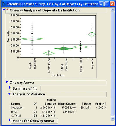
Going back to the Potential Customers data table, Jack and Betty ran the Fit Y by X platform and selected Institution for the X, Factor and Deposits for the Y, Response. This action produces the results in Figure 10.8. Notice that at 10,000 in Deposits (our first vertical reference line in Figure 10.7), most of the observations belong to North Idaho with some in State Employee, a few in Meta Credit, and virtually none in Keystone and Wash Interstate. This corresponds quite well with the probabilities in Table 10.1. There are no observations in North Idaho above about 14,000, which also corresponds well with Table 10.1. In the $50,000 range, virtually all of the observations are in Wash Interstate and Keystone, which again agrees with Table 10.1
Figure 10.8 Analysis of Variance for Deposits Grouped by Institution
Summary
This chapter has introduced the basic concepts of logistic regression, which attempts to predict a qualitative variable, either nominal or ordinal, with a quantitative continuous variable. Although similar in concept to regression analysis as discussed in Chapter 9, logistic regression is very difficult in the mathematical and statistical details. Rather than using the principle of least squares to fit the model and predict an exact value, logistic regression uses maximum likelihood to develop a model to predict a probability ratio. The results of logistic regression are easiest to understand when the Response column has only two values, sometimes called binomial regression. With multiple values for the Response, called multinomial regression, the results are somewhat more complex but follow the same principles.
Chapter Glossary
- binomial regression
- Logistic regression when the Response or dependent variable has only two values.
- logit
- The natural logarithm of an odds ratio.
- multinomial regression
- Logistic regression when the Response or dependent variable has more than two values.
- odds
- A measure of relative likelihood, which is the ratio of one probability to another.
Questions and Problems
Hank Wilson and John Riggins in the Finance Department were discussing the possibility of predicting whether or not someone would take out a loan for a new or used car. They believed that those with more money would be less likely to take out car loans than those with fewer resources. Hank asked John to use the Potential Customers.jmp data to try to predict auto loans from deposits.
1. Conduct the analysis for John. Is there a significant relationship between deposits and auto loans?
2. Using the results from question 1, what is the probability that an individual with deposits of $50,000 would take out a car loan?
Mary Warner, the COO, would like to establish a way of predicting ATM and bill pay usage so that she can predict when usage of these resources might change depending on changing demographics.
3. Conduct the analysis of predicting ATM usage by age. What is the equation for predicting the odds of not using ATMs to using ATMs? Is the relationship statistically significant?
4. Conduct a logistic regression predicting bill pay usage based on age. Are the results statistically significant?
Bob Reed in Human Resources wants to know what drives employees to be on the company health plan and other employees to not be on the plan. Use the Employee Data.jmp data table to answer the following questions for Bob.
5. Can salary be used to predict health plan usage? Are the results statistically significant? What is the probability that an employee making $50,000 will be on the company health plan?
6. Can age be used to predict health plan usage? Are the results statistically significant? What seems to happen to health plan enrollment as age increases?
..................Content has been hidden....................
You can't read the all page of ebook, please click here login for view all page.