

P a r t 2
Visualizing Data: Descriptive Statistics
Exploring Data Using Graph Builder
JMP IN ACTION
Mike Cramer is Director of Operations Research for Worldwide Restaurant Innovation for McDonald’s. Cramer and his colleagues are responsible for helping design and develop McDonald’s restaurants worldwide. His job is to anticipate and monitor trends, identify and analyze opportunities for improvement in operations at McDonald’s, and to advise store owners and others within McDonald’s how to enhance customer service. Among his essential everyday tools is JMP statistical software, which he has been using for four years. One of the main strengths of JMP software, its visualization capabilities, serves as an important communication medium for Cramer in communicating statistical concepts to internal and external clients who have limited statistical knowledge. JMP is primarily used by Cramer’s group for predictive analytics—gathering historical data and then projecting it into the future. Graph Builder is among Cramer’s favorite JMP features because it allows him to easily modify a graph or construct a new one to better understand and communicate trends and patterns in the data. One of his goals is to replace Microsoft PowerPoint presentations with interactive JMP presentations to better handle questions that cannot be anticipated in advance. Rather than having to go back and reanalyze data to answer questions later, the data can be manipulated during the meeting to answer the questions immediately.
Since JMP is visually oriented, it makes sense to start our discussion of statistical techniques with two visual presentation methods, tables and charts. JMP can quickly and easily create numerical tables and is capable of creating a wide variety of different graphs. The analytical methods in JMP routinely include graphics as part of the output. In this chapter, we will focus primarily on creating tables in JMP and the Graph platform that creates specialized graphs.
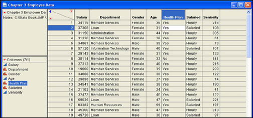
Bob Reed works for Alice Hansen in Human Resources at INCU. Bob and Alice were recently discussing how employees at INCU compared with other financial institutions in the area. Alice asked Bob to take a sample of employee records and develop some tables and graphs that would give them a better picture of the demographic profile of their employees. The structure of the data is shown in Figure 3.1, and the data are contained in the file Employee Data.jmp. For each employee, the data set includes their salary, department in the credit union, gender, age, whether or not they are in the company health plan, whether they are hourly or salaried employees, and seniority with the credit union in months.
Tables are often a clear and forceful method of presenting data. Analytical tables are arranged to show comparisons or relationships. They should convey the writer’s message in a simple and effective manner. Bob needs to create tables for Alice that describe the employees of INCU.
There are two alternative ways of creating tables in JMP, both of which start with the Tables menu.
The first way to create tables in JMP is through the Tables → Summary menu command. This command is a quick way to display summary statistics for a few columns. Bob first decides to look at some summary data for the age of the employees in the sample.
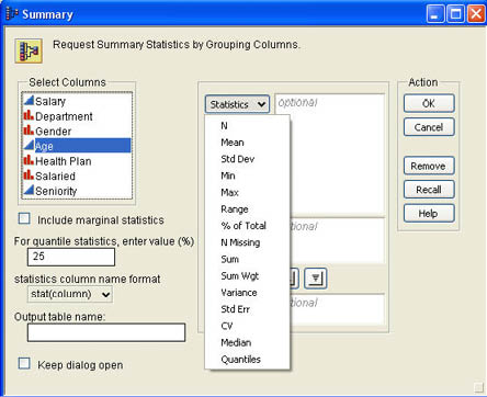
To create the summary table, Bob selects Tables → Summary from the JMP menu. The dialog shown in Figure 3.2 then appears. Bob selects Age from the list of columns on the left side of the dialog. Bob then has to select from a variety of statistics in the Statistics drop-down of the dialog. Figure 3.2 also shows the options available for the statistics. All of these statistics will be described in more detail in Chapter 4. For this chapter, we will use only the first two options: N, which is the number of observations, and Mean, which is the average value. The statistics that JMP will allow you to select depend on the modeling types of the column or columns that you selected in the Select Columns list. For example, if you select Gender, a nominal scale qualitative variable, it will not allow you to select the Mean statistic because this would not make sense for a nominal scale variable. We will have more to say about this issue in the next chapter.
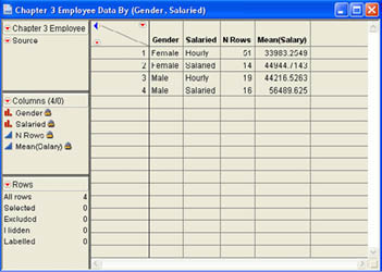
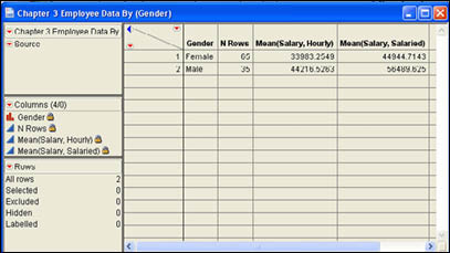
You can also group the statistics by the levels of a nominal or ordinal column. Selecting an appropriate nominal or ordinal column in the Select Columns list and then clicking Group will summarize the data by levels of that column. You can add additional columns to group by in one of two ways. You can select additional nominal and ordinal columns and click Group. This will add those columns to the rows of the results report (Figure 3.3). Alternatively, you can select these columns and click Subgroup. This will add the levels of that column to the columns of the results report (Figure 3.4). Bob decides to look at the average current salaries grouped by Gender with subgroupings based on whether or not they are salaried. The results are shown in Figures 3.3 and 3.4. Notice that the data are not formatted very attractively in the resulting reports. To format the values in a column of the report, double-click the column name to access the Column Info dialog where you can format the data.
You can add additional statistics columns to a report that you have already created. To do this, click the drop-down menu for columns (![]() ) in the report and select Add Statistics Column from the menu. This will produce a dialog similar to that shown in Figure 3.3 except the Group option will not be available. You can select another continuous column to add to the report and select a summary statistic for it.
) in the report and select Add Statistics Column from the menu. This will produce a dialog similar to that shown in Figure 3.3 except the Group option will not be available. You can select another continuous column to add to the report and select a summary statistic for it.
In reading the JMP documentation, Bob has discovered that a more flexible and versatile way to create tables in JMP is with the Tabulate command. This command is accessed by selecting Tables → Tabulate from the JMP menu. This will open a dialog like that shown in Figure 3.5. You can drag-and-drop columns into the row or column zones in the table.
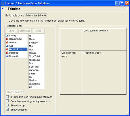
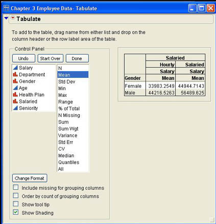
Some of the variables that you drop in the rows or the columns will be grouping variables that will normally be nominal or ordinal type variables. If you drop a continuous variable into the Row or Column drop zones, JMP will ask you if you want to Add Grouping Columns or Add Analysis Columns. Selecting Analysis Columns will place the summary results for that variable into the Resulting Cells area. The default statistic summarized will be the Sum of the values for that column, but you can then drag and drop the statistics you want from the Statistics list to replace that statistic. If at any point you want to scrap what you have done so far and start over, click Start Over in the Control Panel. You can also delete columns from the table by right-clicking on the column name and selecting Delete from the menu. Bob decides to redo the table for average salaries grouped by gender in the rows and the salaried/hourly variable in the columns. The results are shown in Figure 3.6.
After you have completed your table, you may want to hide the control panel. To do this, click the drop-down menu icon (![]() ) from the Tabulate menu and uncheck the Show Control Panel menu item. You can always go back and restore the control panel later by reversing this process.
) from the Tabulate menu and uncheck the Show Control Panel menu item. You can always go back and restore the control panel later by reversing this process.
To add other grouping or analysis columns to the table, drag and drop the names into the appropriate locations. You can also add new summary statistics to the table with the same process.
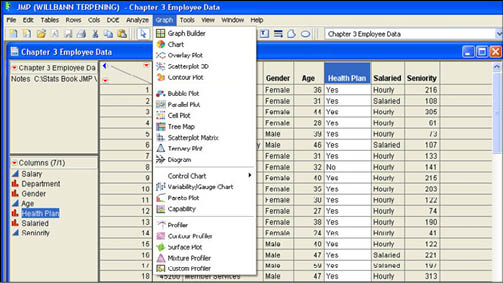
Although graphs and charts are a big part of almost all of the analysis platforms in JMP, a wide variety of graphs and charts can be accessed directly through the Graph menu command. Figure 3.7 shows the menu options available from the Graph menu command. We will consider only some of these options here in this chapter. Also, we will look at other graphic options that are not located under this command. However, this section is a good place to start with the built-in graphic capabilities of JMP.
The first section of menu options contains the most familiar “classic” graphic forms, such as bar charts, pie charts, and line graphs. We will look at several of these options in this chapter. The second group of options contains a set of less traditional, but very useful, graphic options. We will look briefly at a few of these options here, and at least one of them will also be used in later chapters. Since the kinds of graphs that we will discuss are located in different places in JMP, our discussion in this chapter will be organized around the modeling types of columns we are dealing with and what we are looking for in the data. We will first discuss charts most appropriate for qualitative data, i.e., nominal and ordinal data. We will then discuss charts for quantitative or continuous data. Finally, we will examine some special charts and tables that are oriented toward looking at relationships between both types of variables.
Graphs and charts for qualitative data consist of two common charts and one that is likely less familiar to you. These charts are primarily for displaying nominal and ordinal scale variables.
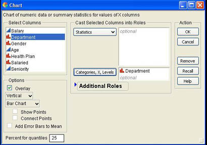
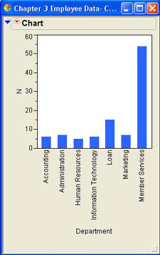
Bar charts are a very familiar way of representing frequencies or count data for nominal and ordinal scales. These charts can be produced in JMP by selecting the Graphs → Charts platform from the menu. The resulting dialog for the employee data is presented in Figure 3.8. To produce a bar chart simply select a column, click on the Categories, X, Levels button, and click OK.
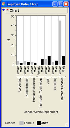
Bob has produced a simple frequency bar chart for Department, which is shown in Figure 3.9. If you would prefer a horizontal bar chart instead of a vertical one, click the drop-down menu icon (![]() ) and select Horizontal Chart. To go back to the vertical arrangement, click the drop-down menu and select Vertical Chart. You can also display multiple columns in a single bar chart. For example, if we select both Gender and Department as category columns, we would obtain the chart shown in Figure 3.10a.
) and select Horizontal Chart. To go back to the vertical arrangement, click the drop-down menu and select Vertical Chart. You can also display multiple columns in a single bar chart. For example, if we select both Gender and Department as category columns, we would obtain the chart shown in Figure 3.10a.
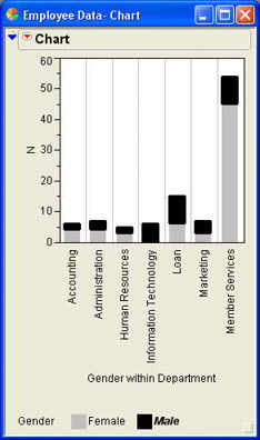
If you prefer a stacked arrangement rather than side by side, click the drop-down menu icon (![]() ) and select Stack Bars to get the results shown in Figure 3.10b. You can unstack the bars by selecting this same option again.
) and select Stack Bars to get the results shown in Figure 3.10b. You can unstack the bars by selecting this same option again.
 (a) Side by Side Bar Charts |
 (b) Stacked Bar Charts |
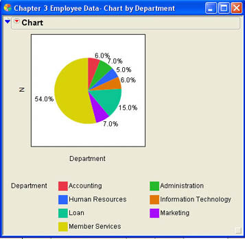
The second very familiar format for qualitative charts is the pie chart, which is especially useful for depicting the relative frequencies for nominal and ordinal data. You can produce pie charts in two ways. First, you can select Pie Chart instead of Bar Chart in the Options section of the Chart dialog shown in Figure 3.8. The second way to produce a pie chart is to first produce the default bar chart and then click the drop-down menu icon (![]() ) and select Pie Chart. The pie chart variant of the Department chart shown in Figure 3.9 is shown in Figure 3.11. The labels in Figure 3.11 have been reformatted using the drop-down Chart menu of the results report.
) and select Pie Chart. The pie chart variant of the Department chart shown in Figure 3.9 is shown in Figure 3.11. The labels in Figure 3.11 have been reformatted using the drop-down Chart menu of the results report.
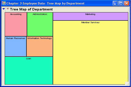
Although not originally developed for this purpose, tree maps can be useful in displaying frequency information for nominal and ordinal scale variables when there are a large number of categories.1 To illustrate the use of tree maps, we will again use the Department variable of our Employee data set. To generate a tree map, select Graphs → Tree Map from the JMP menu. The dialog shown in Figure 3.12 opens. To produce a tree map of frequencies or counts for a qualitative variable, select the column in the Select Columns list, click Categories, and then click OK. The resulting tree map for the Department counts is shown in Figure 3.13. This tree map looks similar to the pie chart but is square rather than round. The real advantage of tree maps is for nominal or ordinal data with a large number of categories where a pie or bar chart would have so many alternatives that it would be very confusing. In these cases, a tree map is a much better choice.
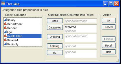
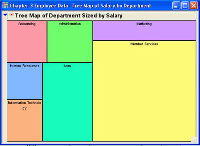
You can also use a continuous variable along with a qualitative variable in a tree map by selecting a continuous column and clicking Sizes. The magnitude of the continuous variable will then determine the size of the rectangle rather than the frequency of the qualitative variable. An example is shown in Figure 3.14, where the salaries of the employees in the department determine the size of the rectangle for each department. A comparison of Figure 3.13 and 3.14 reveals some interesting details. For example, the sizes of the Information Technology and Loan departments are clearly larger when sized by salary (Figure 3.14) than they are when sized by count (Figure 3.13). This indicates higher average salaries in these two departments.
Now we will look at some graphic techniques for quantitative or continuous data. The oldest form of graphical presentation for continuous data is the histogram. Histograms, however, lose information and are therefore not as desirable as more modern presentations such as stem-and-leaf diagrams. Line charts are specialized charts usually used for time series data.
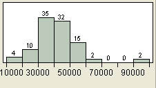
Histograms are basically bar charts for continuous or quantitative variables. However, a bar chart of a continuous variable is not very informative. Recall that a bar chart represents the frequency with which each value occurs. Often for continuous variables, each value occurs only once or twice in the data. For example, with the salary variable in the employee data in Figure 3.1, each value occurs exactly once. A bar chart of this data, shown in Figure 3.15, does not reveal anything useful about potential data patterns. For continuous variables, the data must be grouped in some fashion and then presented as a bar chart. Such a chart is called a histogram. Histograms are produced automatically as part of the Distribution platform for continuous variables. We will discuss this platform in great detail in the next chapter. For now, we will just present the histogram produced by this platform for the salaries in our Employee data. The results are shown in Figure 3.16.

Notice that a histogram is basically a bar chart but that there are no gaps between the bars unless an interval has a frequency of zero. That is because the underlying variable is continuous, unlike the discrete values of the bar chart.
A histogram provides a picture of the general shape of the distribution of values, an idea of the spread of the values, and often an indication of the middle value of the distribution. A shortcoming of the histogram is that it loses information about individual values. For example, we can see from Figure 3.16 that most of the salaries are concentrated around the $30,000 to $50,000 range and there are a few very large salaries of $90,000 or more. However, a general picture of the data is about all that we can garner from a histogram. We even lose the specific information about each observation in the data. For example, we know that there are 36 values in the $30,000 range, but we have no idea what these values are. Are they evenly dispersed across this range, or are most of them located at one end or the other? From a histogram, there is no way to tell. This is why some analysts prefer other graphical techniques that we will discuss in this chapter and the next.
A technique developed by John Tukey (1977) does a good job of describing the general nature of a set of data without losing as much information as we do with a histogram. Stem-and-leaf diagrams represent each continuous value in two parts, a stem and a leaf. Each leaf represents a single digit. A stem many represent multiple digits depending on the magnitude of the values. Stem-and-leaf diagrams are also produced via the Distribution platform. We will demonstrate how to obtain these figures in the next chapter. Here, we will simply look at their interpretation. Figure 3.17 shows the stem-and-leaf diagram for the salaries data. Each observation of the data is represented in the diagram by a stem and a leaf. The stem is on the left side of the dividing line and the leaf is on the right. The legend at the bottom of the chart illustrates the interpretation of the values. The legend indicates that 1|9 represents 19000, the smallest salary. The largest salary is represented as 9|9 is $99,000. Some of the lines represent more than one number. For example, the line 6|033 represents three salaries of $60,000, 63,000, and 63,000. The column on the right gives the count of the number of leaves in each stem of the diagram.
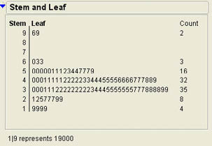
Another way to view a stem-and-leaf diagram is like a histogram turned sideways. For example, we can easily see that the majority of the salaries are in the $30,000 range just from the number of leaves with a stem of 3.
Histograms and stem-and-leaf diagrams are both designed to show the shape, spread, and location of a set of numbers. We have already mentioned that the disadvantage of histograms is that information is lost in the presentation of the data. However, stem-and-leaf displays also have some disadvantages. A major limitation is with large data sets. As implemented by most software, stem-and-leaf diagrams are most useful for smaller data sets and become much less useful for large sets of numbers. Stem-and-leaf displays are generally not recommended for more than 150 observations or so. Histograms should be used for larger data sets.
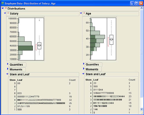
A second disadvantage of stem-and-leaf diagrams in JMP is that they are not interactive like histograms are. This places them at a disadvantage in performing side-by-side comparisons of data. For example, suppose Bob wants to compare the distribution of the salary data with the distribution of the age data. Figure 3.18 shows the histograms derived for the two columns using the Distribution platform. Note the connection between the two histograms in Figure 3.18. When you click on a section of the histogram for salary (the salaries between $30,000 and $40,000), the corresponding data in the Age histogram are also highlighted. When you do this in the histogram, the corresponding data in the stem-and-leaf display are also highlighted as shown in Figure 3.18 but there is no way to do this directly within the stem-and-leaf diagrams.
In general, for large data sets, the histograms are better in JMP. For smaller data sets, it is, like many things visual, a matter of preference with the exception of the interactivity of the histogram.
Line charts are frequently used to depict the values of a continuous variable over time with the time scale on the horizontal axis. They are effective for comparing one time period with the next and for presenting a picture of long-term trends in the series of data. If the time scale does not begin at zero, we must clearly indicate that so as not to mislead the reader. Although the Y axis normally contains the original scale of the variable, sometimes it is better to replace the Y values with their natural logarithms for data that are increasing (or decreasing) at an almost constant rate (as opposed to a constant amount) or for comparing fluctuations in two series where the numbers have vastly different magnitudes.
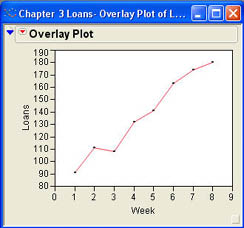
To illustrate line charts, we need time series data. Sarah Schumaker, an analyst in the Loan Department at INCU, has kept track of the number of loans made for the past 8 weeks. The data are shown in Table 2.1 and are also contained in the file Loans.jmp.
| Week | 1 | 2 | 3 | 4 | 5 | 6 | 7 | 8 |
| Loans | 91 | 111 | 108 | 132 | 141 | 163 | 174 | 189 |
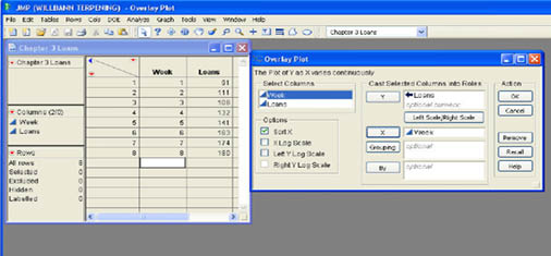
Line graphs can be produced using either Graph Builder or the Overlay Plot platform under the Graphs menu. Graph Builder will be discussed later in this chapter, so we will illustrate the Overlay Plot option here. Selecting Graphs → Overlay Plot from the menu opens a dialog as shown in Figure 3.19, which also shows the data table for this example. The column Week is selected for the X axis, and column Sales is selected as Y.
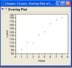
The graph that is produced when you click OK is simply a plot of the points with no connecting line as shown in Figure 3.20a. Select either Connect Thru Missing or Y Options → Connect Points from the drop-down menu in the report table to connect the points with a line as shown in Figure 3.20b. As you can see from the chart, the numbers of loans at INCU have been generally increasing over the last 8 weeks. This is a good trend if INCU is trying to increase their loan volume.
 (a) |
 (b) |
In this section, we want to investigate methods for exploring the relationship between two variables. We will first look at the relationship between two continuous variables measured on an interval or ratio scale, and we will then look at ways of exploring qualitative variables measured on nominal or ordinal scales.
Scatter plots are graphs of two continuous variables. Scatter plots are used to detect if there is a general relationship between the two variables X and Y.
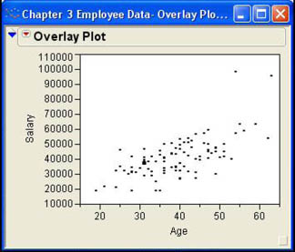
Our employee data for INCU data contained continuous variables for salary and age. One of the things that Alice has asked Bob to do is look at the relationship between salary and age so that they can better plan salaries as their employees age. Logically, we would probably expect a positive relationship between these two variables. Older workers have more experience and are generally paid more because of that.
There are three ways to produce a scatter plot in JMP. You can use the Fit Y by X platform under the Analyze menu, or the Scatterplot Matrix or Overlay Plot platform under the Graph menu. We will work with the Fit Y by X platform in more detail in Chapters 7 through 9. The Scatterplot Matrix platform is primarily designed for examining multiple scatter plots of many continuous variables at the same time. We will find this format useful when we talk about regression analysis in Chapters 9 and 10. For now, we will use the Overlay Plot option that we used for line charts above. The Overlay Plot dialog was shown in Figure 3.19. In our example, we would select the column for seniority, click X, select the salary column, and then click Y. The result is shown Figure 3.21. There does appear to be a positive relationship between the two variables in that as age increases so does salary.
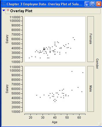
The Overlay Plot platform has the additional benefit that we can graph the scatter plots separately by different groups using a grouping variable. Figure 3.22 shows the results of our scatter plots using gender as a grouping variable. In this figure, we can see that the salaries appear to rise more quickly as a function of age for females than for males. In Chapter 10, we will look at methods for quantifying these relationships so that we can more directly compare them.
Bubble plots are a recent innovation in graphing statistical data that allows the analyst to add additional variables to a basic scatter plot to reveal more information. Visualize a basic XY scatter plot with the points represented by bubbles that can be sized based on a third variable. That is the essential idea of the bubble plot. Select Graphs → Bubble Plot from the JMP menu to launch the bubble plot platform.
The bubble plot dialog is shown in Figure 3.23.
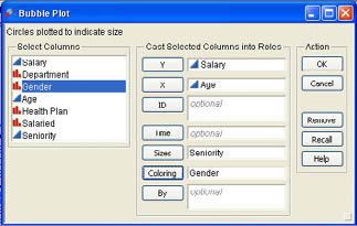
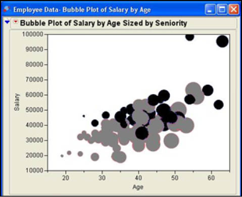
As in the previous example, we will again plot Age on the X axis and Salary on the Y axis. These variables are selected in the same fashion as with the scatter plot above. To size the bubbles, select a column to use in sizing (in our case, we will use Seniority) and then click the Sizes button. You can also use a nominal or ordinal column to produce different colors in the bubbles. In our example, Gender has been picked to color the bubbles. The resulting bubble plot is shown in Figure 3.24. The plot again shows that there is a positive relationship between Age and Salary. In addition, it shows that Gender also impacts salaries. The higher salaries tend to be larger bubbles. It also shows that male salaries, shown in black, tend to be somewhat higher than female salaries, shown in gray.
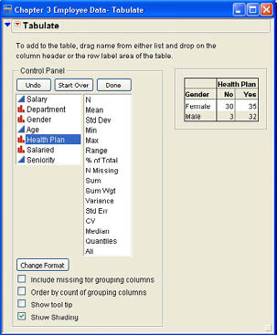
When we have nominal or ordinal columns, we should not display relationships between the variables as a scatter plot since scatter plots assume that the variables are continuous—i.e., measured at on at least an interval scale of measurement. In fact, JMP will not allow you to place a nominal variable as the Y value in an overlay plot. To explore relationships between nominal or ordinal scale data, the correct technique is the contingency table. A contingency table is simply a table of frequencies or counts where the rows and columns of the table are the nominal or ordinal scale categories. Contingency tables can be produced using either the Tables → Tabulate or Tables → Summary methods described earlier or with the Fit Y by X platform. Of the three, the Tabulate method is the simplest.
Bob Reed wants to know whether there is a relationship between gender and participation in the company health care plan. Since these variables are clearly nominal scale measures, a contingency table would be the appropriate means of exploring the relationship between the two variables. Figure 3.25 shows the Tabulate dialog and the resulting contingency table when Gender is used as the row and Health Plan is used as the column. As you can see from the figure, there tends to be a relationship between gender and the use of the health plan in that males overwhelmingly tend to use the health plan, but females are almost evenly split on whether or not they use the plan. In other words, based on these data, it appears that the two variables are not independent of one another, but whether or not one uses the company health plan tends to depend on gender. We will make further use of contingency tables in Chapters 8 and 9 to explore the effects of nominal scale variables.
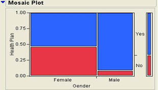
A mosaic plot is simply a plot divided into rectangles where the area of each rectangle is proportional to the frequency of that category. Mosaic plots can be used to depict a single nominal or ordinal variable as we will discuss in the next chapter. However, these plots may be most useful in exploring the relationships between two qualitative variables. A mosaic plot will be produced in the Fit Y by X platform when both X and Y are nominal or ordinal variables. Bob again wants to look at the relationship between Gender and Health Plan. He selects Analyze → Fit Y by X from the JMP menu. The resulting dialog is shown in Figure 3.26.
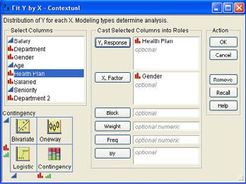
He selects Gender in the Select Columns section and clicks X, Factor. Then he selects Health Plan and clicks Y, Response. Finally, he clicks OK to perform the analysis. The mosaic plot portion of the results table is shown in Figure 3.27. The rest of the output from this analysis will be discussed in Chapter 9. As with the contingency table, we can clearly see that females are about evenly split on whether or not they are enrolled in the health plan while males are overwhelmingly enrolled in the plan.
One of the major design features of the JMP software is the belief in the importance of exploring data to get a better understanding of the information that the data contains. One of the most intuitive ways that humans deal with numerical information is with graphs, and the graphical capabilities of JMP are ideal for this purpose. In this section, we will illustrate the process of exploring data using the Graph Builder platform of JMP. To illustrate exploring data through the use of graphs, we will utilize an example from the JMPer Cable magazine.2 At its world headquarters in Cary, North Carolina, SAS now has two solar farms in operation. The first started operation in January 2009. Data for this example were gathered at the first farm from January to August of 2009, and the output of the farm was measured separately for two halves of the farm called Array A and Array B. The first example will look at the power output from the two Arrays over time of day. To load Graph Builder, select Graph → Graph Builder from the JMP menu. Figure 3.28 shows the Graph Builder dialog with the columns from the solar farm data.
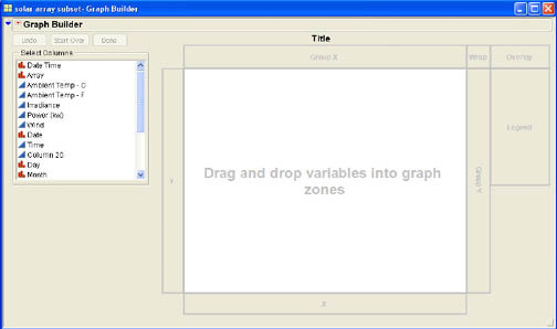
In some ways, Graph Builder is similar to the Tabulate command for building tables described earlier in this chapter. Similar to Tabulate, the dialog here contains drop zones. To build a graph all that is required is to drag column names and “drop” them (by releasing the mouse button) into the appropriate zones of the dialog.
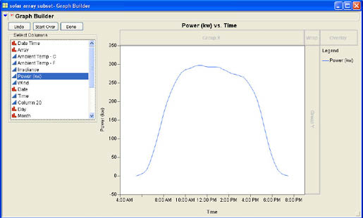
For this graph, we want Time to be the X variable and Power to be the Y variable, so we drag the column names to the appropriate locations. At this point, we have a simple graph showing the increase in power generated as the sun rises in the morning toward its peak around noon and the decline toward evening hours as shown in Figure 3.29.
There are four other drop areas in Graph Builder. These drop areas use nominal or ordinal columns to create graphs separately for each of the values of that column. The first drop area that we will use is the Overlay area. When you drop an appropriate column into the Overlay area, JMP creates a separate graph on the Y axis for each value of the overlay column. We will use the Array column to create separate graphs for the two different arrays. Figure 3.30 shows the resulting graphs.
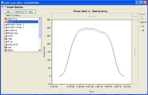
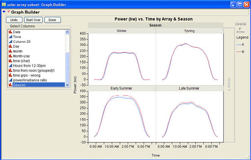
As you can see from the graphs, during the peak period. Array B generates slightly more power than does Array A. It is not immediately obvious why this should be the case. We can further explore the data by using the other three drop areas in Graph Builder. There are two Group drop areas, one for the X axis and one for the Y axis. As with the Overlay area, we will normally drop nominal or ordinal columns into these areas to create separate graphs for the different levels of the Group variable. A column dropped in the Group X area will create a new X axis for each level of the grouping column. Similarly, dropping a column into the Group Y area will create a separate Y axis for each value of the grouping column. If you wish to recreate both the X and Y axis for each level of the grouping column, then you should drop the grouping variable into the Wrap area in the upper right corner of the dialog. In the solar panel data, there is a column called Season that groups the data into 2-month groupings, January–February, March–April, May–June, and July–August. We will use this variable as a Wrap variable. Dropping Season into the Wrap area produces the four graphs shown in Figure 3.31. As you can see, the gap in power production between Array A and Array B does not exist in the Winter or Spring season but only in the Early Summer and Late Summer. This means that there is something that has a differential impact on the two different arrays during these times. The article in JMPer Cable further explores these differences.
As you can see from this simple example, Graph Builder is a powerful tool for exploring data graphically and provides a number of different options, not all of which we have shown here.
Data are raw materials that must be processed in order to produce useful information. Tables and charts are visually oriented devices used to summarize and make sense out of data. The particular tables or charts used depend on the modeling type of the variables (nominal, ordinal, or continuous) and on whether we are looking at the individual variables (univariate analysis) or at relationships between variables (bivariate analysis).
Qualitative data can be displayed in tables, bar charts, pie charts, or tree maps. Quantitative variables are typically displayed as histograms, stem-and-leaf diagrams, or line charts. Stem-and-leaf diagrams are similar to histograms but do not lose the original information as do histograms. However, stem-and-leaf diagrams do not scale well with large data sets, and histograms have an additional advantage of dynamic linking in JMP.
Relationships between variables can be explored by using scatter plots or bubble plots for continuous variables, or with contingency tables for nominal and ordinal data. Graph Builder provides a ready platform for graphically exploring a set of data.
In Chapter 2, we described the situation of Ann Thompson, Director of Marketing for Olin Garden Supply, Inc. Ann has information on 40 customers gathered over the past year. For each customer, she has information on the zip code where they live, number of people in the household, whether or not they used a credit card for purchases, whether or not they purchased live plants, and amount purchased from Olin during the past year. The data are contained in the file Olin Gardins.jmp.
1. Generate a bar chart showing the number of customers by zip code. Where do most of Olin Garden’s customers come from?
2. Generate a mosaic plot of the customers by zip code. Which chart do you prefer, bar chart or the mosaic plot? Discuss why you prefer one over the other.
3. Display a stem-and-leaf diagram of sales for Olin Gardens.
4. Show a contingency table of customers by zip code and whether or not they used a credit card for purchases. Does the use of credit cards vary by zip code?
5. Develop a table of average sales by zip code. Which zip code generates the highest average sales?
Bill McDuffey needs to generate some tables and charts for his boss for an upcoming executive meeting. Using the Bullseye.jmp data from Chapter 2, develop the following tables and charts for Bill.
6. Bill needs a table of average sales by sales region. Develop the table for Bill.
7. Bill thinks that departmental sales may differ by region. For example, the department with the top sales in one region may not be the top department in another region. Develop a table for Bill exploring the sales by region and department. What conclusions can you draw from this table?
8. Bill’s boss wants to know if there is a relationship between household sales and sales of women’s apparel. Develop the appropriate chart for him. Does there appear to be a relationship between the two? If so, is the relationship positive or negative?
9. Bill thinks that the relationship between household sales and women’s apparel may depend somewhat on the size of the store. Develop a bubble plot for Bill where the size of the bubble represents the size of the store. What can you tell Bill from this plot?
10. Bill notices that there is not a variable for total sales for each store. Add such a variable to the data table. Show a stem-and-leaf diagram for total sales. What would be a good value to represent “average” sales for the stores?
Tukey, John W. 1977. Exploratory Data Analysis. Reading, MA: Addison-Wesley.
1 Tree maps were developed by Ben Shneiderman at the University of Maryland to display hierarchical data, originally for displaying files in a computer directory structure. For more information see http://www.cs.umd.edu/hcil/treemap-history/.
2 This article appeared in the Winter 2010 edition of JMPer Cable which can be downloaded from http://jmp.com/about/newsletters/jmpercable/index.shtml. The data for this example can be downloaded from this same location.