
The Fit Y by X Platform for Qualitative Variables
The Logic of Chi-Square Tests for Contingency Tables
Contingency Tables and the Classic Z Test
In this chapter, we will deal exclusively with qualitative variables that are either primarily nominal scale or occasionally ordinal scale variables. With qualitative variables, we can no longer talk about means or variances but are restricted principally to frequency counts or proportions. With two qualitative variables, the frequencies are typically presented in contingency tables. A contingency table is simply a table of frequency counts where the rows and columns of the table are both qualitative variables. Contingency tables are commonly used for two purposes. The first is to test for a relationship or association between two qualitative variables. Such tests are commonly called tests of independence. We will not discuss this type of test in this chapter. The second use of contingency tables is as a test of proportions. In the special case of two rows or two columns, the statistic of interest is usually the proportion of observations that fall into one particular row or column. Here we will resume our discussion of proportions that we skipped in Chapter 7. Another way of looking at this chapter is that it is similar to Chapter 7 where the Y or Response variable is a qualitative variable rather than quantitative.
The Situation at INCU
The Executive Council at INCU consists of Susan Strong (CEO), Hank Wilson (CFO), Darrell Young (CTO), Mary Warner (COO), Alice Hansen (Vice President of Human Resources), and Ann Rigney (Vice President of Marketing). This group has had several discussions over the past few months about how they can increase their market share in terms of members in their existing geographical locations. They have decided that they really need better data about potential customers who are currently banking with other institutions. They have asked Ann Rigney and her Marketing Department to begin a study of potential customers that will give them some hard data on which to base their decisions.
Ann has asked Betty Anderson and Jack Snowden to take the lead on designing and administering the survey. Betty and Jack, in consultation with others in the Marketing Department have come up with a questionnaire design, and with Ann’s agreement they plan to gather the following information: which financial institution the customers are currently using; are they happy there (Yes/No); are they familiar with INCU and its services (Yes/No); do they use ATMs (Yes/No); do they use electronic bill pay (Yes/No); their current satisfaction with each of these services; their technical expertise (Novice, Intermediate, Expert); their age; and the approximate amount currently deposited with their primary financial institution. Because of the sensitivity of some of the information being sought, Betty and Jack agree to gather the information through personal interviews with a randomly selected sample of potential customers who are not currently customers of INCU.
The Fit Y by X Platform for Qualitative Variables
As with the last chapter, the primary platform for our analyses is the Fit Y by X platform. You can access this platform either through the JMP Starter or through the JMP menu. Using the JMP Starter, you can access this platform through the Basic group by selecting Contingency. Optionally, you can click Fit Y by X, and JMP will automatically determine the type of analysis depending on the nature of the columns you pick to analyze.
Example 8.1
Betty and Jack have now completed their survey of 200 potential customers in Washington and Idaho. The data have been compiled into a data table named Potential Customer Suvey.jmp, parts of which are shown in Figure 8.1
Figure 8.1 Potential Customer Survey Data Table
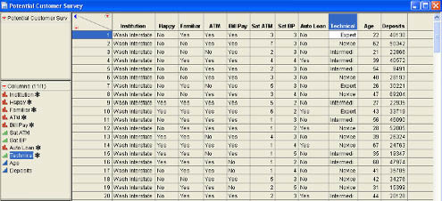
Most of the columns in the data table are character in nature. The two satisfaction measures (Sat ATM and Sat BP) and the Technical measure have been set to ordinal, and Age and Deposits are both continuous. Betty and Jack first decide to perform an analysis of financial institutions (Institution) and how happy the individuals are with that institution (Happy). Jack loads the data table Potential Customers.jmp and selects Analyze → Fit Y by X from the JMP menu. In the dialog, he selects Happy as the Y, Response and Institution as the X, Factor. In other words, Jack and Betty are going to look at the effect of financial institution on how happy the customer is. After Jack clicks OK, they observe the results window shown in Figure 8.2. This figure shows only part of the initial output. We will discuss all sections of the results as we progress through the chapter.
Figure 8.2 Partial View Preliminary Results for Example 8.1
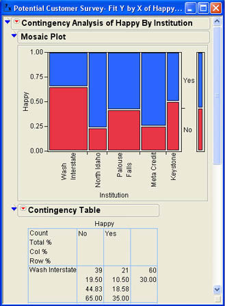
The first part of the results window is a Mosaic Plot as first introduced in Chapter 3. The plot has the Factor column on the X axis and the Response column on the Y axis. The area of each rectangle shows the percentage of the observations in each category for that column of the Factor. The last column on the right shows the overall proportion of each level of the Response column. In this case, slightly over 50% said yes and a little fewer than 50% said no. For the financial institutions, it can quickly be seen that Washington Interstate had the largest percentage of no responses and North Idaho had the smallest percentage of no responses, and therefore the largest proportion of yes responses. The second section of the results window is the Contingency Table. The full table is shown in Figure 8.3.
Figure 8.3 Contingency Table for Example 8.1
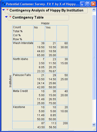
In each cell of the table, the first value is the count or frequency for that cell. For example, the 39 in the first cell of the table indicates that 39 of the respondents with accounts at Washington Interstate responded no to the question of whether they were happy with their financial institution. The second value is the percent of the total count for that cell. In the first cell, 39 is 19.5% of 200. The third value is the percent of the column total represented in that cell. For the first cell 39 is 44.83% of 87. The last value in each cell is the percent of the row total represented in that cell. For the first cell, 39 is 65% of 60. This tells us that 65% of the Washington Interstate members in the sample responded no and 35% responded yes. The marginal totals are also given for each row and each column along with the respective percent of the total number of observations. From the contingency table, we can quickly see that the yes/no responses are not distributed the same way for each financial institution.
You can control what is included in the contingency table using the Contingency Table options by selecting from the drop-down menu (![]() ) as shown in Figure 8.4. To illustrate the logic of the chi-square analysis, we will need to change the values displayed in the contingency table. We will unselect the Total% and Col% options and select the Expected, Deviation, and Cell Chi Square options, which will produce the contingency table shown in Figure 8.5. The next section will describe what these values represent.
) as shown in Figure 8.4. To illustrate the logic of the chi-square analysis, we will need to change the values displayed in the contingency table. We will unselect the Total% and Col% options and select the Expected, Deviation, and Cell Chi Square options, which will produce the contingency table shown in Figure 8.5. The next section will describe what these values represent.
Figure 8.4 Contingency Table Options Menu
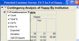
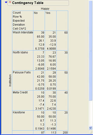
Figure 8.5 Contingency Table after Changing Options
The Logic of Chi-Square Tests for Contingency Tables
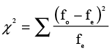
As you may recall, we have used the chi-square distribution before to represent the sampling distribution for a sample variance. We used that distribution to derive confidence intervals and test hypotheses about a single population variance. Hypothesis testing in contingency tables is also done with the chi-square distribution, but it is a very different use of that distribution.1 The chi-square value for contingency tables is based on the deviation of the actual frequencies from the expected frequencies. The equation for the test statistic is
 (8.1)
(8.1)
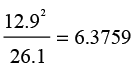
where fo and fe are the observed and expected frequencies respectively, and the summation is over all cells in the table. This is quite different from the equation for the variance described in Equation 5.12. The revised contingency table in Figure 8.5 shows the observed frequency as before, the expected frequency as the second value in each cell, the row percentages that represent the proportions, the deviation or difference between observed and expected frequency for that cell, and the cell chi-square value. When we look at the first cell, the observed frequency is 39, the expected frequency is 26.1, and the deviation is 12.9 so that the cell chi-square is
To see the logic of the chi-square test, let’s consider a likely hypothesis test for this situation. Since there are two values for the Response column, the proportion is likely the statistic of interest. Our hypothesis is therefore about a population proportion. In this case, we have five different levels of the Factor column or five different groups. This hypothesis is analogous to our null hypothesis for analysis of variance, so we can formulate it as
H0: π1 = π2 = π3 = π4 = π5
HA: not (π1 = π2 = π3 = π4 = π5)
We can now see where the expected frequencies come from. To illustrate, we will use the first cell in the table; this represents a No response to Washington Interstate. The overall proportion of no responses across all groups is 87 out of 200 or 43.5%. Since the null hypothesis says that the proportion is the same for all groups, under the null hypothesis, we would expect 43.5% of the 60 respondents for Washington Interstate to say no, which is (.435)(60) = 26.1, which is the expected frequency. The other expected frequencies can be calculated with similar logic. For example, in the second cell, we would expect (1 - .435)(60) = 33.9 for the Yes responses for Washington Interstate.
This explains the logic of the expected cell frequencies, but, in practice, they are calculated in an equivalent but much simpler manner. Letting Ri represent the total frequency for the row, Cj be the total frequency for the column, and Total be the overall total number of observations, the expected cell frequency is calculated as
 (8.2)
(8.2)
Using Equation 8.2, we would calculate the expected frequency of the first cell of the table as (60)(87)/200 = 26.1.
We are now ready to look at the final portion of the results window for our analysis. This portion labeled Tests contains the statistical tests needed to test the hypothesis above. This section of the results is shown in Figure 8.6.
Figure 8.6 Tests Portion of the Results Window
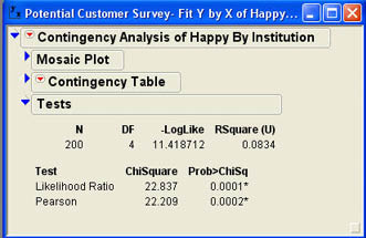
The first part of the output shows the overall number of observations (200) and the degrees of freedom. For a contingency table, the degrees of freedom are the (number of columns – 1)(number of rows – 1) or (5-1)(2-1) = 4 in this case. The next value (-LogLike) is a negative of a log likelihood and is a measure of uncertainty, which we will not detail here. The RSquare (U) value is a value between 0 and 1 that measures the percentage of the categorical response classification correctly predicted by our model, in this case a little over 8%.2 The most relevant part of the output here is the table of test values. There are two chi-square tests shown in the results window. The first is a likelihood ratio test, also sometimes called the G Test. The second, called the Pearson chi-square test, is the one based on our description above and the one most commonly cited in the business literature. Usually the results of these two tests will be very similar. In this case, both tests indicate that we can reject the null hypothesis, which says the proportions are equal in the five groups.
You may wonder if there are comparable multiple comparison tests for proportions like those for means in the analysis of variance. There is a procedure developed by Leonard Marascuilo to perform multiple comparisons for proportions.3 The JMP script accompanying the text will perform the Marascuilo tests. This script shows that the proportion of Yes responses at Washington Interstate (35%) is significantly lower than all other institutions except for Keystone. Also, North Idaho has a significantly higher proportion of Yes responses than does Keystone or Washington Interstate.
Correspondence Analysis
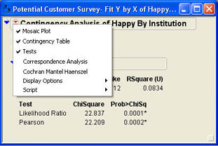
When one of the columns in a contingency table has a large number of levels, interpreting the results presented in the contingency table can be difficult. Correspondence Analysis is an option in JMP which shows which rows or columns in the contingency table have similar patterns of frequency counts. This option can be accessed via the pull down menu for the Contingency Analysis report as shown in Figure 8.7.
Figure 8.7 Contingency Analysis Option Menu
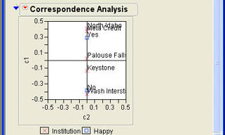
When this option is selected, a graph such as that in Figure 8.8 will be added to the results window. The graph in Figure 8.8 clearly shows that North Idaho and Meta Credit have a high proportion of Yes responses, Washington Interstate has a high proportion of No responses with Palouse Falls and Keystone in the middle.
Figure 8.8 Correspondence Analysis Report
Two by Two Contingency Tables
Two-by-two contingency tables are a special case of the more general situation that we have addressed so far. There are some additional features in JMP for this special case that we will cover in this section. We will first begin with an example.
Example 8.2
Tom Herman in the Information Systems Department at INCU has heard that Marketing has gathered data for a sample of people on whether they use ATMs and bill pay. He asks Jack to help him find out what the data tells him about the relationship between ATM use and bill pay use. In particular, he wants to know if the proportion of people who use bill pay is the same for those that use ATMs and those that do not. In other words, he is interested in testing the following hypotheses:
H0: π1 = π2
H1: π1 ≠ π2
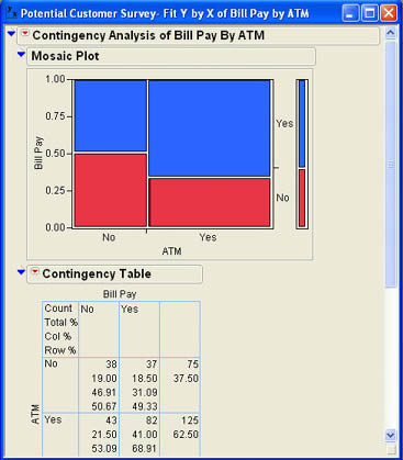
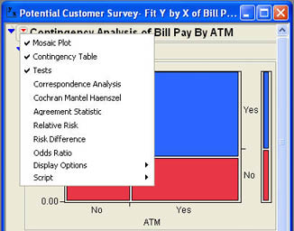
Jack tests the hypothesis for Tom using the Fit Y by X platform and enters the ATM column as the X, Factor and the Bill Pay column as the Y, Response. After clicking OK, Jack views the results shown in Figure 8.9. Jack can see from the Mosaic Plot that the proportion of Yes responses appears to be larger for those who responded Yes to the ATM use question than those that responded No. However, he also knows that this could be due to sampling error and that he needs to look at the hypothesis test results. Scrolling down, he finds the Tests results shown in Figure 8.10.
Figure 8.9 Initial Results for ATM Use and Bill Pay
From the Tests results, he can see that both chi-square values are highly significant so that he can safely reject the null hypothesis and can report to Tom that those who use ATM machines are significantly more likely to use bill pay than those that do not.
Figure 8.10 Test Results Window for ATM Use and Bill Pay
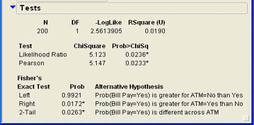
Jack also notices that there is extra output in the Tests results section that was not there in the previous analysis. Also shown in the results section is the Fisher’s Exact Test.
The Likelihood Ratio and Pearson tests are approximate chi-square tests and are most appropriate for large samples. For small samples, Fisher’s Exact test should be used. However, this test is most commonly calculated only for 2 X 2 tables, and that is the only time it is calculated in JMP. When Fisher’s Exact test is given in the output it should be used for the hypothesis test as it is the most appropriate. In this case, Fisher’s Exact test also indicates a significant difference with a slightly higher p-value (.0263).
Contingency Tables and the Classic Z Test
Those familiar with the business statistics literature will know that the test for two population proportions is also often done using the normal distribution and the Z test. Although this test is not an option in JMP, this is not a problem because, as we will see, the Z test is basically equivalent to the Pearson chi-square test for two-tailed tests.
The Z tests statistic for two proportions is
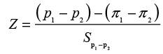 (8.3)
(8.3)
where (π1 - π2) is normally hypothesized to be 0 and the standard error term is calculated using the pooled sample proportion. Since we are not interested in the hand calculations in this text, we will just state the following results:
Z = 2.2687 and p-value = .0233
Notice that the p-value is identical to that obtained for the Pearson chi-square. Also note that if you square the Z value you get 5.147, which is the Pearson chi-square value. Thus these results are entirely equivalent.
Some would argue, however, that the chi-square test can be used only for two-tailed tests and the Z test can be used for one-tailed tests. However, the Fisher Exact test can be one-tailed and is generally preferred in these situations. Therefore, there is no need for the Z test for two population proportions, and we will not discuss it any further here.
Risk Difference
There are four other options available under the Contingency Analysis drop-down menu for two-by-two tables that were not there before. If you compare the options menu shown in Figure 8.11 (from Example 8.2) with that shown in Figure 8.7 (from Example 8.1), you will notice that there are four additional options here: Agreement Statistic, Relative Risk, Relative Difference, and Odds Ratio. We will discuss only the Risk Difference option here.
Figure 8.11 Contingency Analysis Options Menu for Two-by-Two Table
The risk difference is simply the difference between two proportions. When Jack selects Risk Difference, the results shown in Figure 8.12 are appended to the results window.
Figure 8.12 Preliminary Risk Difference Results
The first thing that Jack notices is that he should have been more careful in labeling the outcomes for his qualitative columns. Given that the two columns have identical labels, it is very difficult to determine what the results are telling him. Returning to the data table, Jack right-clicks in the ATM column, selects Column Info, and changes the labels to 0=Don’t Use ATM and 1=Use ATM to be more clear about the values. After making similar changes to the Bill Pay column, he reruns the analysis and again selects the Risk Difference option. The revised results are shown in Figure 8.13 where for convenience the contingency table is also shown but the other parts of the results window are closed.
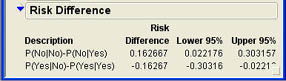
Figure 8.13 Revised Risk Difference Results
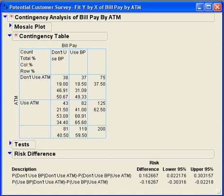
The results are presented in terms of differences in conditional probabilities. Since the conditional event is the Factor column, which is the row of the contingency table, the conditional probabilities can be read from the Row % values of the table. For example, the first risk difference is the Row % value for the first cell of the table (.5067) minus the Row % value for the third cell of the table (.34340) for a difference of .16267. The other risk difference is the difference between the corresponding values in cells 2 and 4.
To see what the risk difference value is really telling us, let’s go back to our original null hypothesis.
where the first group consists of those who do not use ATMs and the second group consists of those who use ATMs. The first risk difference is the difference between the sample proportion in each group that do not use bill pay, and the second risk difference is the difference between the sample proportion in each group that used bill pay. If we regard using bill pay a “success,” then the second risk difference says that:
p1 – p2 = .4933 - .6560 = -.162667
The test results, as we have already seen, tell us that this difference is statistically significant. The Risk Difference analysis also gives us a confidence interval for the difference between the two population proportions, which is from -.30316 to -.02218. This implies that the margin of error is approximately .14 or 14%.
Summary
In this chapter, we examine the Fit Y by X platform where both the Factor and Response columns represent qualitative variables. The logic of chi-square tests for contingency tables is detailed in terms of a test for two or more proportions analogous to the one-way analysis of variance for Chapter 7. Correspondence analysis is a graphical device that is useful when there are a large number of levels of either the Response or Factor variables and helps show relationships between the levels or which levels group together in terms of having similar frequency patterns.
The special case of two-by-two contingency tables is examined and compared to the classic Z test for the difference between two proportions. The Risk Difference analysis of JMP provides an estimate of the difference between the two proportions from the sample along with a 95% confidence interval.
Chapter Glossary
- contingency table
- Table of frequencies where both the rows and columns of the table are qualitative variables.
- correspondence analysis
- Graphical display that groups similar frequencies together to show relationships between levels of the response and factor columns.
- Fisher’s exact test
- Calculates an exact p-value for two-by-two contingency tables.
- Marascuilo tests
- Multiple comparison tests for three or more proportions.
- risk difference
- The difference between two sample proportions.
Questions and Problems
Darrell Young, the CTO at INCU, thinks that the use of online bill pay is related to the technical expertise of the use, but that use of the ATM is not related to technical expertise.
1. Do the data support Darrell’s beliefs about the use of ATMs and bill pay?
The Executive Council is interested in other differences between the competing financial institutions that can be gleaned from the data. In particular, they want to explore the following questions:
2. Are there differences between the financial institutions in terms of the familiarity with INCU and its services? Which institutions have members that are most familiar with INCU and therefore may be more likely to switch?
3. Are there differences between the financial institutions in terms of the use of ATMs or bill pay? Which institutions have the highest usage rates of each technology?
4. Are there differences in the proportion of members who have auto loans between the financial institutions?
5. Does the proportion of members who are happy with their financial institution depend on their level of technological expertise?
References
Marascuilo, Leonard A. 1966. Large-sample multiple comparisons. Psychological Bulletin 65(5), 280–290.
Notes
1 As we will see throughout the remainder of the text, probability distributions are often used for very different purposes in statistics. Tests of variances and tests of contingency tables are only two uses of the chi-square distribution. There are other uses as well.
2 In contingency tables, R Square values are rarely very large.
3 L.A. Marascuilo (2000).
..................Content has been hidden....................
You can't read the all page of ebook, please click here login for view all page.