2.6 Clustered Network

2.6.1 Clustering Coefficient

Highly connected subnetworks are embedded in real-world networks by groups and modules. To measure the clustering effects, the clustering coefficient [18] was proposed. This measure denotes the density among neighbors of node i, and is defined as the ratio of the number of edges among the neighbors to the number of all possible connections among the neighbors:

(2.19)

where M_i is the number of edges among the neighbors of node i (see Fig. 2.7). The overall tendency of clustering is measured by the average clustering coefficient . A high average clustering coefficient implies that the network is clustered.

Figure 2.7 The clustering coefficients of node i with degree of 3 (i.e., k_i = 3).

In random networks, since the probability that an edge is drawn between a given node pair is p, the clustering coefficient is equivalent to the probability p (the model parameter) C^rand = p. Assuming that real-world networks are randomly constructed, the clustering coefficient is estimated as

(2.20)

where E and N are the number of edges and nodes, respectively.

However, the clustering coefficients of most real-world networks are higher than their expected value (see Table 2.2 and Refs. 2,7,18 for details), indicating that the ER random network is not clustered.

The BA model networks are also not clustered, and their clustering coefficient (see Refs. 15,16 for derivation) is

(2.21)

Since the average degree k is expressed as 2m, the clustering coefficient is rewritten as

(2.22)

This clustering coefficient is a bit higher than that of random networks because of the presence of hubs. In the BA model, a newly added node is likely to connect to high-degree nodes selected by the preferential attachment mechanism. When considering the preferential selection of two nodes, the possibility that two selected nodes are connected is relatively high because these nodes have many neighbors. If the added node connects to such a node pair, the number of edges among neighbors increases, leading to higher clustering coefficients. However, the increase in clustering coefficient due to this process is very small (i.e., (ln N)²); thus, the clustering coefficient rapidly decays with increasing N.

In addition, the average clustering coefficient C^nc of random networks with a given degree distribution (e.g., the configuration model) [17,22] is estimated as

(2.23)

The lattice networks are useful for explaining highly clustered networks. For example, the clustering coefficient of each node is 0.5 (= [2 × 3]/[4 × 3]) in a one-dimensional lattice (Fig. 2.3a). This model implies that the constraint of space dimensions contributes to the network clustering observed in real-world networks.

2.6.2 Watts–Strogatz Model

The ER random network model and lattice network model describe the small-world networks and clustered networks, respectively. However, real-world networks possess both statistical properties.

To fill the gap between model networks and real-world networks, Watts and Strogatz [18] proposed a simple network model (referred to as the Watts–Strogatz (WS) model).

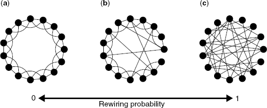
The WS model network is constructed as follows: (i) a one-dimensional lattice is prepared (Fig. 2.8a). (ii) A node and the edge connecting it to its nearest neighbor are selected in a clockwise sense. (iii) With the probability p, the edges are rewired and a new target node selected at random. The processes (ii) and (iii) are repeated until one lap is completed.

Figure 2.8 Schematic diagram of the Watts–Strogatz model.

The model networks are similar to random networks when p = 1. That is, the WS model expresses the transition from lattice networks to random networks, and it includes the random network model and the lattice network models.

Small-world and highly clustered networks emerge when the probability p is in-between 0 and 1 (e.g., 0.01 < p < 0.1). This is because the rewiring of edges is a short-cut path in a lattice network. As mentioned above, lattice networks represent a large average path length; however, the short-cut paths help decrease the average path length. Since the decay of the clustering coefficient by rewiring is slower than that of the average path length, the WS model reproduces small-world and highly clustered networks. However, the node degree follows a normal-like distribution because new target nodes are randomly selected when rewiring an edge, indicating that the WS model does not correspond to a scale-free network.

In addition, the analytical solutions of statistical properties such as clustering coefficient and average shortest path length by changing the rewiring probability p are described in Refs. [23,24]