2.9 Assortativity

The relationship between the degrees in a connected node pair is very interesting. Since real-world networks are nonrandom, we can expect this relationship to be significant. However, degree distribution only involves the degree of each node. Thus, we need an alternative measure for characterizing such a relationship of degrees.

2.9.1 Assortative Coefficient

To characterize the relationship between node degrees, Newman proposed the assortative coefficient [33], defined as

(2.28)

where k_i and k_j are the degrees of two nodes at the ends of an edge, and denotes the average over all edges. This is simply the Pearson correlation coefficient of degrees between a connected node pair, and it lies in the range −1 ≤ r ≤ 1.

The relationship between the assortative coefficient and network structures is described as follows:

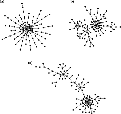
Figure 2.12 Schematic diagram of an assortative network (a), a random network (b), and a disassortative network (c). The networks consist of 100 nodes.

It is generally known that social and technological networks exhibit assortativity and that biological and ecological networks exhibit disassortativity [33].

2.9.2 Degree Correlation

Assortativity relates to the degree correlation. The degree correlation characterizes the expected degree of the neighbors of a node with degree k and is defined as

(2.29)

where Γ_i denotes the average nearest-neighbor degree, expressed as

(2.30)

where V(i) corresponds to the set of neighbors of node i.

That is, the positive and negative degree correlation indicates assortativity and disassortativity, respectively.

In many real-world networks, it is empirically known that degree correlation follows a power–law function:

(2.31)

where ν is a constant, and it also characterizes the assortativity.

The exponent ν takes values −1 < ν < − 0.5 in technological networks such as Internet and the World Wide Web [34,35] and biological networks such as protein–protein interaction networks [35,36] and gene regulatory networks [37]. On the other hand, a positive ν value is observed in social networks such as coauthor networks [35].

Assortativity and disassortativity is never observed in random networks. The degree correlation, Equation 2.29, is also expressed as

(2.32)

where P(k'|k) is the conditional probability that the edge belonging to a node with degree k points to a node with degree k ' [38]. Since networks are randomly constructed, the conditional probability P(k'|k) is k ' × N_k'/[2E], where N_k' is the number of nodes with degree k ' and is equivalent to N × P(k '). E denotes the number of edges. Thus, we obtain

(2.33)

indicating that the degree correlation is independent from the node degree k (i.e., the network shows no assortativity). Since the random network models (i.e., the ER model and the BA model) are randomly constructed, such networks also show no assortativity although the degree distributions are different between these models.

2.9.3 Linear Preferential Attachment Model

To generate assortative and disassortative networks, the linear preferential attachment (LPA) model [39] is useful. This is an extended BA model, and the preferential attachment mechanism is modified as

(2.34)

where a is a constant and ∑_j(k_j + a) = (2m + a)t. This model is equivalent to the BA model when a = 0. When a→ ∞, the probability Π^LPA corresponds to the random attachment mechanism in which nodes are selected with the probability 1/N(t), where N(t) is the total number of nodes at time t. High-degree nodes are more frequently chosen when a < 0. Since networks grow when a is larger than −m, which is the initial degree of a newly added node, the constant a lies in the range −m< a < ∞.

The degree distribution is obtained from the time evolution of the node degree, which is expressed as . Solving this equation, we have

(2.35)

where s is the time at which node i is added. Therefore, the degree distribution in the LPA model follows the power law (scale-free property):

(2.36)

This model has a tunable degree exponent that depends on a and m, although the degree exponent of the BA model is fixed, that is, γ = 3.

The LPA model generates assortative and disassortative networks with positive a and negative a(> − m), respectively.

To show this, we need to consider the time evolution of R_i = ∑ _hV(i)k_h. In this model, there are two conditions for the increase of R_i, as follows:

i. Node i is selected with the probability .

ii. The neighbors of node i are selected with the probability .

In the case of (i), R_i increases by m. In the case of (ii), R_i increases by 1. Thus, the time evolution of R_i is

(2.37)

The first and final terms of the above equation correspond to the increments in conditions (i) and (ii), respectively.

Substituting the solution of the above equation in Equation 2.30, the degree correlation is obtained (see Ref. 15 for derivation). The degree correlations are different with respect to the constant a as follows:

(2.38)

As shown in Equation 2.38, the LPA model generates assortative, random, and disassortative networks depending on the parameter a. In addition, for −m < a < 0, it is found that the exponent of the power–law degree correlation (ν) relates to the degree exponent (γ), that is, ν = 3 − γ.

2.9.4 Edge Rewiring Method

The rewiring based on node degrees [40] is also employed when generating assortative and disassortative networks.

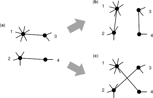
The procedure is as follows. (i) Generate random networks with a given degree distribution by network models (e.g., the configuration model introduced in Section 2.4.5). (ii) Two edges are randomly selected, and the four nodes are ranked in order of their degrees (Fig. 2.13a). (iii) When generating assortative networks, the highest degree node is connected to the next highest degree nodes (Fig. 2.13b). In contrast, for disassortative networks, the highest degree node is connected to the lowest degree node (Fig. 2.13c). In both cases, the other edge is drawn between the two remaining nodes.

Figure 2.13 Schematic diagram of rewiring based on node degrees. The integer corresponds to a rank order based on node degrees. (a) Two randomly selected edges. (b) Rewiring for assortative networks. (c) Rewiring for disassortative networks.

Steps (ii) and (iii) are repeated until the rewiring of all edges is completed.