5.2 Methods
5.2.1 C3NET
5.2.1.1 C3NET (Conservative Causal Core)
C3NET consists of three main steps [12]. The first step is for estimating mutual information for all gene pairs. In the second step, the most significant link for each gene is selected. In the third step nonsignificant links, according to a chosen significance level α, between gene pairs are eliminated. The inferred link in a C3NET gene regulatory network correspond to the highest MI value among the neighbor edges for each gene. This implies that the highest possible number of edges that can be inferred by C3NET is equal to the number of genes under consideration. This number can decrease for several reasons. For example, when two genes have the same edge with maximum MI value. In this case, the same edge would be chosen by both genes to be included in the network. However, if an edge is already present another inclusion does not lead to an additional edge. Another case corresponds to the situation when a gene does not have significant edges at all. In this case, apparently, no edge can be included in the network. Since C3NET employs MI values as test statistics among genes, there is no directional information that can be inferred thereof. Hence, the resulting network is undirected and unweighted. Figure 5.1 shows the principle working mechanism of C3NET. The maximum mutual information value between gene 7 and 5 (dashed line) is not significant. All other genes have significant MI values. This results in a total of 7 edges in the inferred network. As one can see, the structure enabled from this can assume an arbitrary complexity and is not limited to simple connections among genes. The reason for this is that the selection of genes (left-hand side) is directed, whereas the final network (right-hand side) is an undirected network. For a more detailed technical explanation of C3NET, the reader is referred to Ref. [12].
Figure 5.1 Principle working mechanism of C3NET. The MI value between gene 7 and 5 (dashed) is not significant.
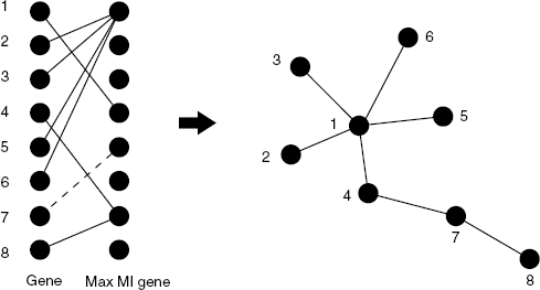
In contrast, common mutual information-based gene regulatory network inference approaches RN [17], ARACNE [18], or CLR eliminate nonsignificant links for all possible gene pairs. This leads to more extensive computational effort and is often circumvented by applying arbitrarily chosen fixed significance thresholds. However, the C3NET approach allows to infer a gene regulatory network without any predefined threshold for the significance of the mutual information.
5.2.2 Estimating Mutual Information
In this chapter, we study the influence of the statistical MI estimator of mutual information values on the inference of regulatory networks. We investigate four different types of estimators that are based on the so-called histogram approach. In the first step, the expression values of two genes are discretized into defined intervals denoted as bins. Mutual information is a measure for the nonlinear dependence between two random variables. Mutual information is defined by the joint probability P(X, Y) of two random variables X and Y[19]. We compute mutual information by
(5.1) ![]()
I(X, Y) is always ≥0 and we use base 2 for the logarithm. Mutual information can also be calculated from the marginal and joint entropy measures of the random variables X and Y:
(5.2) ![]()
The marginal entropy for a random variable X is defined by
The joint entropy H(X, Y) is defined by
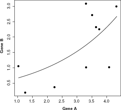
In the following, we give a numeral example how the mutual information is computed using the empirical MI estimator for an artificial expression profile for two genes. As example, we generated a linearly dependent expression profile for two genes (Fig. 5.2).
Figure 5.2 Example for correlated gene expression for two genes (10 samples). The expression values for gene A are sampled from a normal distribution with μ = 3 and σ = 1 and the expression values for gene B are defined by gene A with an additional noise ![]() sampled from a normal distribution with μ = 0 and σ = 1.
sampled from a normal distribution with μ = 0 and σ = 1.
We use three different discretization methods. The first, equal frequency method requires the same number of values in each bin. The second, equal width method defines the interval for each bin with the same size and the third, global equal width method is similar to equal width. Here, the intervals are defined for both random variables simultaneously, rather than separately for each random variable. We use k-proportional interval discretization method [20] that defines the number of bins in dependency of the sample size by ![]() . In Table 5.1, we use the global equal with the method to discretized the expression profile for two genes. From the discretized values the count frequencies define the empirical joint probability for each value occurring in the defined intervals can be described for gene A and gene B by the joint probability matrix P(x, y) (Table 5.2).
. In Table 5.1, we use the global equal with the method to discretized the expression profile for two genes. From the discretized values the count frequencies define the empirical joint probability for each value occurring in the defined intervals can be described for gene A and gene B by the joint probability matrix P(x, y) (Table 5.2).
Table 5.1 Continuous and Discretized Gene Expression Profile of Gene A and Gene B.

Table 5.2 Empirical Joint Probability Matrix is Obtained from the Joint Count Frequencies of the Two Expression Profiles for Each Bin.

The marginal entropies for gene A and gene B are calculated using Equation (5.3):

From the discretized expression profiles, the joint probability for each defined bin is empirically computed from the observed frequencies for gene A and gene B:
using Equation (5.4) the joint entropy is then computed by
![]()
Hence, we obtain the following Mutual information:
![]()
We describe four different strategies for estimating mutual information for a discretized model. The simplest estimator is the empirical estimator that assumes normality for the values that fall in each bin. However, the main problem with this approach is that the values are often nonuniform distributed among the bins that lead to a skewed estimate of mutual information. A variety of approaches were developed to account for the induced bias that range from correcting the estimate by a constant factor or using a multivariate distribution to model the extend of missing information. In the following, we show four different mutual information estimators that are based on a discretized model. Note that the formulas for the shown estimators are for a single random variable.
The empirical MI estimator gives the maximum likelihood estimate and is based on the observed count frequencies for the values in a bin as shown in the example (see Table 5.2), where the entropy is estimated from the empirical probability distribution with nk being the number of samples in bin k and N is the total number of samples.
![]()
The empirical estimator gives an underestimate of entropy due to the undersampling of bins when the number of bins B is large. The Miller–Madow estimator [21] accounts for this bias by adjusting the MI estimate by a constant factor proportional to the number of bins and samples.
![]()
Here B is the number of bins and N the number of samples.
The shrinkage estimator [22] combines two models for defining cell probabilities, one model with a cell probability of ![]() and the empirical model with a cell probability
and the empirical model with a cell probability ![]() .
.
![]()
The λ parameter is estimated by minimizing the mean squared error for the two models for each k of B bins.
![]()
The entropy for the shrink estimator is computed by
![]()
The Schürmann–Grassberger [23] uses a Dirichlet probability distribution as conjugate prior. The Dirichlet distribution is a multinomial distribution with mean values θk.
![]()
The average θk are computed from the posterior using the maximum-likelihood function of the empirical estimator and the Dirichlet prior. The posterior with Schürmann–Grassberger parameters ![]() equals
equals
![]()
Note that one pseudocount is added in overall to all bins (N + 1). The entropy is computed by
![]()
5.2.3 Global Measures
In the following, we describe global error measures to evaluate the performance of the inferred network. The most widely used statistical measures are obtained by comparison of an inferred (predicted) network with the true network underlying the data. From the measures listed below, three pairwise combinations thereof are frequently used to assess the performance of network inference algorithms. In the following, we show quantities that are estimated from relations between the number of true positives, true negatives, false positives, and false negatives.
The recall, also known as sensitivity, denotes the proportion of true positive inferred edges relative to all edges in the reference network.
(5.5) ![]()
The precision gives the proportion of correctly inferred edges relative to all inferred edges.
(5.6) ![]()
The specificity is a measure for the relative proportion of edges which were correctly rejected.
(5.7) ![]()
The complementary sensitivity is a measure for the proportion of falsely inferred edges.
(5.8) ![]()
The accuracy measures the overall proportion of true edges of the reference network to all falsely inferred and true edges.
(5.9) ![]()
Mutual information-based network inference algorithms obtain a rank for each predicted edge denoted by a rank statistic or the MI estimate as for example used in C3NET. The inferred network is obtained by a defined threshold θ ![]() Θ for the rank statistic of the edges. When the true network is known the threshold that gives the best inference performance can be defined by quantifying the global proportions of true and falsely predicted edges. The first global measure we describe is the area under the curve for the receiver operator characteristics (AUC-ROC) [24]. The ROC curve represents the sensitivity (true positive rate, TPR) as function of the complementary sensitivity (false positive rate, FPR) obtained by using various threshold values θ
Θ for the rank statistic of the edges. When the true network is known the threshold that gives the best inference performance can be defined by quantifying the global proportions of true and falsely predicted edges. The first global measure we describe is the area under the curve for the receiver operator characteristics (AUC-ROC) [24]. The ROC curve represents the sensitivity (true positive rate, TPR) as function of the complementary sensitivity (false positive rate, FPR) obtained by using various threshold values θ ![]() Θ. For each threshold θ, a confusion matrix is obtained that contains the number of true positive, false positives, true negatives, and false negative predictions. The ROC curve of a good classifier is shifted to the upper left side above the main diagonal that shows higher true positive than false positive predictions.
Θ. For each threshold θ, a confusion matrix is obtained that contains the number of true positive, false positives, true negatives, and false negative predictions. The ROC curve of a good classifier is shifted to the upper left side above the main diagonal that shows higher true positive than false positive predictions.
The second measure is the AUC-PR (area under the precision-recall curve) that is obtained similarly as AUC-ROC. The PR curve represents the precision (predicted true positives) as function of the sensitivity (recall, true positive rate). In contrast to the AUC-ROC curve the AUC-PR shows for a good classifier a convex curve shifted to the upper right side showing increase of precision and recall performance. The AUC-ROC area under the curve value is computed by a numerical integration along each point of the curve.
When the rate of positive and false positives or precision and recall are equal the classifier predicts as good as a random guess. This corresponds to a diagonal line along the ROC or PR space. An AUC-ROC or AUC-PR value of 0.5 corresponds to a classifier performing as good as a random guess.
The third measure is the F-score that describes a weighted average of the precision and recall.
(5.10) ![]()
also called F1 because it is a special form of
(5.11) ![]()
The performance measure is obtained by the maximal F-score. This leads to a θ-dependence of all quantities listed above and, hence, allows to obtain a functional behavior among these measures.
We want to emphasize that all measures presented above are general statistical measures used in statistics and data analysis. None of them is specific to our problem under consideration, namely, the inference of networks. Further, all of these measures can only be applied to data for which the underlying network structure is known, because the true network is needed for calculating the above measures.
5.2.4 Ensemble Data and Local Network-Based Measures
In contrast to the above measures, which were global measures, we present now local network-based measures introduced recently [25, 26]. These local network-based measures are based on ensemble data and the availability of a reference network G that represents the “true” regulatory network. Ensemble data means that there is more than one dataset available from the biological phenomenon under investigation. This ensemble could be obtained either by bootstrapping from one large dataset, from a simulation study or by conducting multiple experiments.
After the ensemble of data ![]() is obtained, application of an inference algorithm results in an ensemble of estimated networks
is obtained, application of an inference algorithm results in an ensemble of estimated networks ![]() (Fig. 5.3). Here, we emphasize that each dataset depends on the underlying network structure G that governs the coupling among the genes by writing, for example, Di(G). Further, this indicates that always the same network G is used. From the ensemble of estimated networks
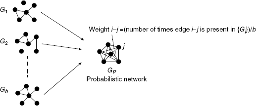
(Fig. 5.3). Here, we emphasize that each dataset depends on the underlying network structure G that governs the coupling among the genes by writing, for example, Di(G). Further, this indicates that always the same network G is used. From the ensemble of estimated networks ![]() one obtains one probabilistic network GP. This network is a weighted network and the weight of each edge is defined by
one obtains one probabilistic network GP. This network is a weighted network and the weight of each edge is defined by
(5.12) ![]()
It is easy to see that ![]() corresponds to the probability that edge eij is present in
corresponds to the probability that edge eij is present in ![]() ,
,
(5.13) ![]()
The aggregation of an ensemble of networks to obtain the probabilistic network ![]() is visualized in Figure 5.4.
is visualized in Figure 5.4.
Figure 5.3 Schematic visualization of ensemble data of which networks are inferred and subsequently aggregated to estimate a probabilistic network.
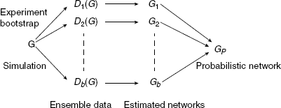
Figure 5.4 The ensemble of networks {Gi} is used to obtain a weighted network GP.
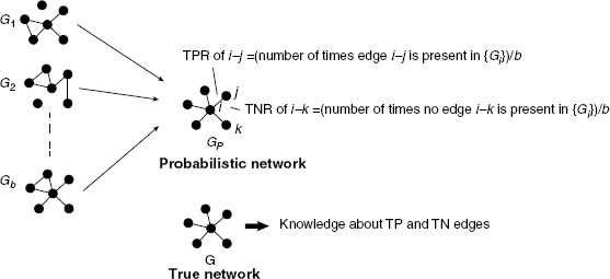
If the network structure of the underlying network G is available it is possible to obtain estimates of the TPR and TNR of edges and nonedges in G. For example, if there is an edge between gene i and j in G we obtain,
If there is no edge between gene i and j in G we obtain instead,
This is visualized in Figure 5.5. It is important to realize that the network G is here used to classify edges/nonedges to different edge sets. Such a classification is not possible without G. From Equations (5.14) and (5.15), follow the corresponding negative rates by
and, hence, all statistical measures described in Section 5.2.3. However, it should be emphasized that now, not the global inference performance with respect to the entire network is characterized but of individual edges. To make this clear, we are calling such measures local network-based measures [25,26]. The Equations (5.14)-(5.17) provide the finest resolution obtainable because an edge is the most basic unit in a network.
Figure 5.5 If the true network G is used in addition to the ensemble of networks {Gi} one obtains estimates for the TPR and TNR of all edges.
A practical consequence of the information provided by {TPRij} and {TNRij} is that it is possible to construct further local network-based measures representing larger subparts of a network. For example, one can construct measures to characterize the inferrability of network motifs consisting of n genes or the influence of the degree of genes. Principally, any combination of {TPRij} and {TNRij} values would result in a valid (statistical) measure, for example, of network motifs. Further examples of such measures can be found in Refs. [25,26].
In order to make the basic principle behind such a construction of local network-based measures more clear, we present as an example motifs consisting of three genes. Recently, it has been recognized that network motifs are important building blocks of various complex networks, including gene networks [27-30]. For this reason, biologically, it is of interest to study their inferrability. Formally, we define the true reconstruction rate of a motif by
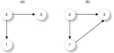
Here, TPR corresponds either to a TPR if two genes are connected or to a TNR if these genes are unconnected and the factor results from the fact that we consider three-gene motifs only, however, extensions thereof are straightforward. Figure 5.6 illustrates two examples of three-gene motifs. From Equation (5.18), we obtain for these two motifs
(5.19) ![]()
(5.20) ![]()
Each of these measures represents the inferrability of a certain motif type. Averaging over all motifs of the same type found in network leads to the mean true reconstruction rate ![]() of a certain motif type.
of a certain motif type.
Figure 5.6 Two examples of three-gene network motifs.
5.2.5 Local Network-Based Measures
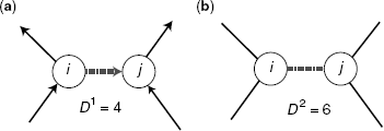
The most frequently studied local structural properties of biological networks are, for example, network motifs, node degree classes, and community structures. In this section, we will address the influence of different mutual information estimators on local network-based measures. The local measure is based on the estimated true positive rate (TPR) of the inferred edges from the ensemble. We demonstrate the structural influence on the true positive rate (TPR) using binary classification of the edges according to the degree of the nodes enclosing an edge. From the ensemble the TPR weights for the edges are compared between two classes defined from the degree of their nodes. We introduce a local measure for directed and undirected networks that are defined by the measure D1 and D2.
The measure D1 is defined for a directed graph as the sum of the out-degree of node i plus the in-degree of node j:
(5.21) ![]()
A binary classification of the edges is obtained by assigning edges to two classes of edges, depending on the value of D1. Specifically, for D1 the classes are defined by
- Class I: Edges with D1 ≤ 3 (corresponds to a chain-like structure)
- Class II: All other edges
The measure D2 is defined for an undirected graph by the sum of the degrees of node i plus the degrees of node j:
(5.22) ![]()
As shown above for D1, a binary classification of the edges is obtained by assigning edges to two classes of edges with a high graph density score and a low graph density score. For D2 the classes are defined by
- Class I: Edges with D2 ≤ 4 (corresponds to a chain-like structure)
- Class II: All other edges
An example is shown in Figure 5.7, for the directed measure D1 and the undirected measure D2. We measure the influence of mutual information estimators on the two defined edge classes. The ensemble of networks is inferred from bootstrap expression datasets to estimate the TPR (see Section 5.2.4). From the ensemble, we obtain the distribution of the mean TPR for the two classes of both measures in D1 and D2 that are compared.
Figure 5.7 An edge (dashed) is scored according to the degree of the adjacent nodes for (a) directed network (sum of out degree i and in degree j) and (b) undirected network (sum of degree i and degree j).
5.2.6 Network Structure
The structure of networks can be described by homogeneous networks and inhomogeneous networks [31]. Homogeneous networks belong to the class of exponential networks such as the Erdös and Rènyi [32], [33] and Watts and Strogatz graph model (Small-World) [34], where all nodes in the network have approximately the same number of edges [31]. Inhomogeneous networks belong to the class of scale-free networks in which the number of edges for the nodes follow a power–law distribution [35]. This property allows the network to contain highly connected nodes such as network hubs [31].
We study the influence of the network structure on the C3NET inference using random networks with different values of p. Here, p is the probability for the presence of an edge between the two nodes. Because real gene networks, for example, the transcriptional regulatory network or the protein network, are sparse the value of p needs to be chosen to fall within a realistic interval. Typically, gene networks are sparse with an edge density of about ![]() 10−3 [36].
10−3 [36].
For our study, we are using networks with n = 150 genes resulting in a maximal number of E = 22, 350 (directed) edges. We generated three Erdös–Rènyi graphs with edge density ![]() = {0.003, 0.006, 0.008} with {22, 19, 10} unconnected nodes. The networks are shown in Figure 5.8. For the number of edges E
= {0.003, 0.006, 0.008} with {22, 19, 10} unconnected nodes. The networks are shown in Figure 5.8. For the number of edges E![]() the density of a graph is defined by
the density of a graph is defined by ![]() = E
= E![]() /E with the number of edges E
/E with the number of edges E![]() = {77, 145, 170}.
= {77, 145, 170}.
Figure 5.8 Three Erdös–Renyi networks with edge density ![]() = {0.003, 0.006, 0.008}.
= {0.003, 0.006, 0.008}.

A broad collection of procedures for in silico gene expression simulation are available, for example, GeneNetWeaver [37], NetSim [38], SYNTREN [39] for time-course and steady-state experiments that are used to validate the network inference accuracy. For our study, we generate simulated steady-state gene expression datasets. Gene expression datasets were simulated using SYNTREN [39] with the bionoise parameter set to 0.05. In SYNTREN, gene expression is modeled using nonlinear Michaelis–Menten kinetics with a superposed function that models biological noise not related to the experiment.
