6.6 Tuning Topology Generator Parameters
The aim of this section is to examine how well the topology generators match the Skitter topology for different values of their parameters. To facilitate this comparison, grids are constructed over the possible values of the parameter spaces and various cost functions are evaluated as follows:
(6.20) ![]()
(6.21) ![]()
(6.22) ![]()
In addition to examining different parameter values across a grid, the optimum parameters with respect to C3(θ) are estimated using the Nelder Meade simplex search algorithm [36,37]. Note that the topologies generated by the topology generators are random in a statistical sense, due to differing random seeds for each run. Ten topologies are generated for each value of θ and the average spectral distribution is calculated. We found that the variance of the spectral distributions was sufficiently low to allow reasonable estimates of the minima in each case.
6.6.1 Link Densities
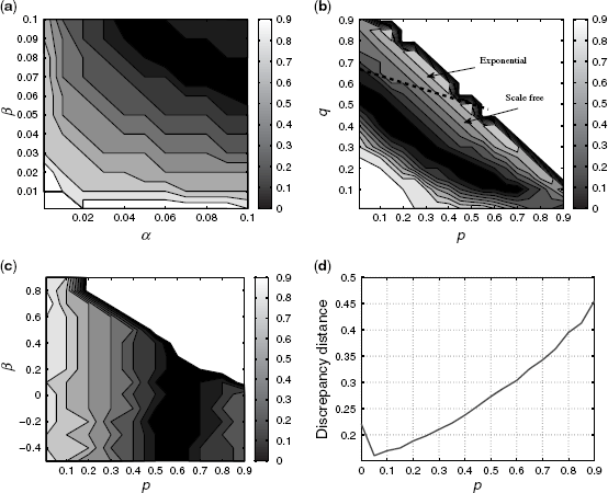
Figure 6.12 displays the value of the cost function C1(θ) as a function of the topology generator parameters. On the upper and lower left graphs, the grayscale color indicates the value of the cost function. For Inet there is only one parameter, p, so it is plotted as a curve in Figure 6.12d. Figure 6.12 shows that a minimum exists for each topology in approximately the same regions as the default values of each generator.17 For the BA generator, it is known that for values of p and q above the line shown in Figure 6.12b, the topologies generated follow an exponential node degree distribution while those below follow a scale-free distribution. It is encouraging to note that the values of C1(θ) are large in the exponential region and the minimum is in the scale-free region as the node degree distribution of the Internet is known to be approximately scale free [11]. Overall the results obtained by tuning the parameters based on C1(θ) appear reasonable. For link density matching it is possible to obtain parameter values which match the link densities exactly. Indeed, there is a ridge of parameters for BA, GLP, and Waxman for which the link densities can be matched. However, as noted in the introduction, there is no control over any other characteristic of the graph using this method.
Figure 6.12 Topology generator parameter grid for sum-squared error from number of links. (a) Waxman. (b) BA. (c) GLP. (d) Inet.
6.6.2 Spectra PDF
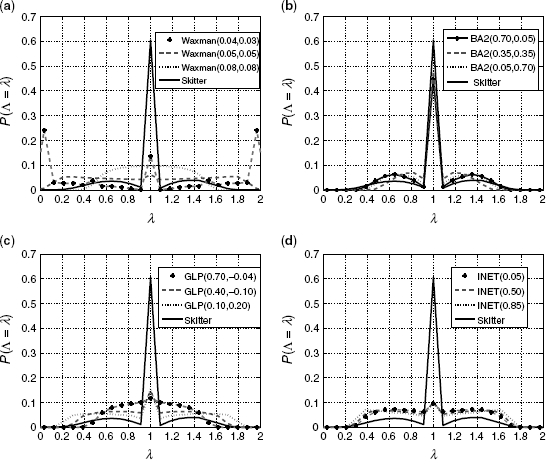
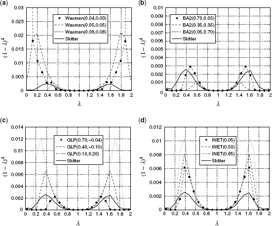
Figure 6.13 shows the spectral PDF of the Skitter dataset and the four topology generators calculated at three parameters values in each grid (the parameter values are indicated in brackets in the legends). The aim is to illustrate how much the spectral PDFs change with the values of the parameters. The spectral PDFs of Waxman (Fig. 6.13a) vary significantly for different values of α and β. Furthermore, none of the Waxman PDFs match well with the spectral PDF of the Skitter graph. The BA PDFs vary to a lesser extent (Fig. 6.13b) and appear to give a much better match than the Waxman model, especially around eigenvalue 1 (λ = 1). This better match of BA is not surprising as the Waxman model is not a good model for the Internet as noted in Section 6.5. GLP (Fig. 6.13c) and Inet (Fig. 6.13d) give similar results to BA, with a poor match outside eigenvalue 1. The better match of the BA model around eigenvalue 1 is interesting. As noted in Section 6.2 the regions away from eigenvalue 1 are far more important than the region around λ = 1. However, what is required is a technique that reveals the differences with distance from one as these are more important. Thus, it would appear difficult to evaluate which model, or even which parameter, is better based on the PDFs alone. This point is now further explored by analysis of the grids calculated with respect to C2(θ).
Figure 6.13 PDF of spectra. (a) Waxman. (b) BA. (c) GLP. (d) Inet.
6.6.3 Limitations of Spectra PDF
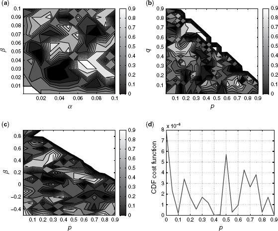
Figure 6.14 shows the value of the second cost function C2(θ) as a function of the topology generator parameters, in the same way as Figure 6.12. As can be seen in Figure 6.14, there are many islands corresponding to local minima, creating a rugged landscape. The variance in the PDFs referred to in this section is actually greater than any gradient that might exist in the grid. This means that it is not possible to estimate the minimum with respect to C2(θ). Figure 6.14 shows that the spectrum on its own is not sufficient to identify the optimum parameters of any of the topology generators. This is because each eigenvalue in C2(θ) is weighted equally. As noted in Section 6.2, the eigenvalues close to 1 are more likely to be affected by the random seeds for each topology generator and are the source of the noise on the grid.
Figure 6.14 Parameter grid for sum of absolute differences of spectra CDFs. (a) Waxman. (b) BA. (c) GLP. (d) Inet.
6.6.4 Weighted Spectra
The previous section illustrated the limitations of using the raw eigenvalues to find optimal topology generator parameters to match the Skitter topology. Figure 6.15 shows a plot of the weighted spectra of the same topologies as those shown in Figure 6.13. As can be seen the results are quite different from those shown in Figure 6.13. The Waxman weighted spectra still shows a bad fit with respect to the Skitter data (mainly around 0 and 2) compared to the other generators. The other generators (BA, GLP, and Inet) now show that they are capable of matching the weighted spectra of the Skitter topology, especially around the point of greatest weight (λ = 0.4 or 1.6). The difference between the weighted spectra around 1 is no longer of importance (in contrast to Fig. 6.13), reflecting that the weights here approach zero as we approach eigenvalue 1. In the next section, the optimum values and the resulting weighted spectra will be compared.
Figure 6.15 Weighted spectra grid for generator parameters. (a) Waxman. (b) BA. (c) GLP. (d) Inet.
6.6.5 Weighted Spectra Comparison
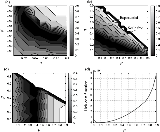
Figure 6.16 shows the grids associated with C3(θ). As can be seen the grids show that there is a region with a minima in each case and in addition, comparing Figures 6.16 and 6.12 it can be seen that these minima lie in a region close to those for C1(θ). However, it should be noted that the weighted spectra will try to fit more than just the number of links in a topology. This demonstrates the inherent trade-off. Also of note is that the region of interest for the BA model lies inside the region of scale-free behavior as shown in Figure 6.16b.
Figure 6.16 Grid of sum-squared error of weighted spectra for topology generators. (a) Waxman. (b) BA. (c) GLP. (d) Inet.
