7.6 Empirical Data

One might argue that our conclusions are based on asymptotic expansions only, thus it is not certain if the observations hold for practical relevant settings. To overcome this weak point, we obtained numerical results that are provided in this section.

We start providing some results concerning the phase transition and the “critical” value ε = 0, for ordinary and symmetric bipartite graphs. Recall that the latter value corresponds to the relation m = n, that is the number of edges equals half the number of nodes. From Theorem 7.2.1, we conclude that the probability that no complex component occurs drops from to . The numerical results given in Table 7.2 exhibit a similar behavior, see also Tables 7.4 and 7.5. Note that the observed number of complex components is slightly below the expectation calculated using the asymptotic approximation. However, the accuracy increases as the number of nodes increases.

Table 7.2 Number of Graphs Containing a Complex Component out of 5 × 10⁵ Graphs Generated for Each Setup.

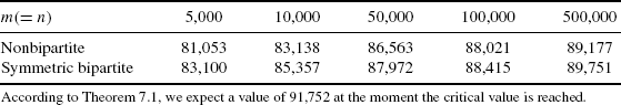
Table 7.4 The Excess of the Complex Part of a Symmetric Bipartite Graph Possessing m Nodes of Each Type and n = (1 − ε)m Keys.

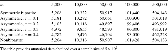
Table 7.5 The Excess of the Complex Part of a Nonbipartite Graph Possessing 2m Nodes and n = (1 − ε)m Keys.

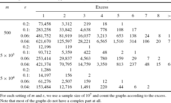
Table 7.3 provides the numerically obtained average number of edges at the moment before the first bicyclic component is created. From the data given in Table 7.3, we conclude that this number is only slightly larger than m, except if the asymmetry is increased. Due to Ref. [13], we know that the first bicyclic component of a usual random graph appears at “time” , what is in accordance with our numerical results. Moreover, we conjure that the same (or a very similar) result holds for the bipartite graph too. Concerning asymmetric cuckoo hashing, we observe that the asymmetry reduces the critical ratio of edges and nodes that determines the start of phase transition.

Table 7.3 Average Number of Edges at the Moment When the First Bicyclic Component Occurs.

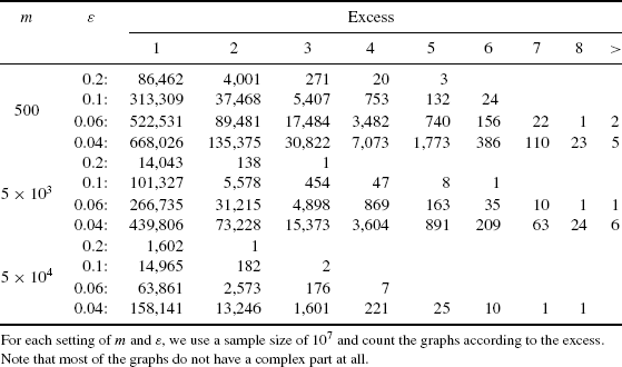
Next, we consider the complex part of the graph in the subcritical phase. Recall that we consider the excess of this part of the graph, that is, how many more edges than nodes it contains. From Theorem 7.2.1, we deduce that the probability that this number equals r is given by . Thus, we expect an exponentially decreasing pattern. The corresponding results are depicted in Tables 7.4 and 7.5. From the data given in both the tables, we additionally observe the following properties: for fixed r > 0 and m, the percentage of graphs with excess r increases as ε decreases. On the other hand, increasing m while holding ε constant, is likely to decrease the excess. Note that these numerical results are in good accordance with the theoretical analysis. Comparing the two different graph models, we observe that the symmetric bipartite case usually leads to a lower occurrence of all positive values of excess. Again, this corresponds well to the findings of our asymptotic analysis.

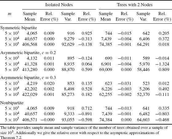
Table 7.6 displays the average number of trees of size one (isolated nodes) and two counted during 10⁵ experiments. Further, we consider several different models, including some asymmetric bipartite settings. Recall that higher asymmetry leads to a lower maximum load factor, hence some small values for ε would be invalid for some asymmetric settings. From the data given in Table 7.6, we see that our asymptotic results are good approximations. In particular, we observe that the symmetric bipartite and the ordinary model do not only share the same limiting distribution concerning the number of trees, they also exhibit a indistinguishable behavior in practice. However, we deduce that asymmetry increases the number of isolated nodes.

Table 7.6 Number of Trees of Sizes One and Two for ε = 0.1.

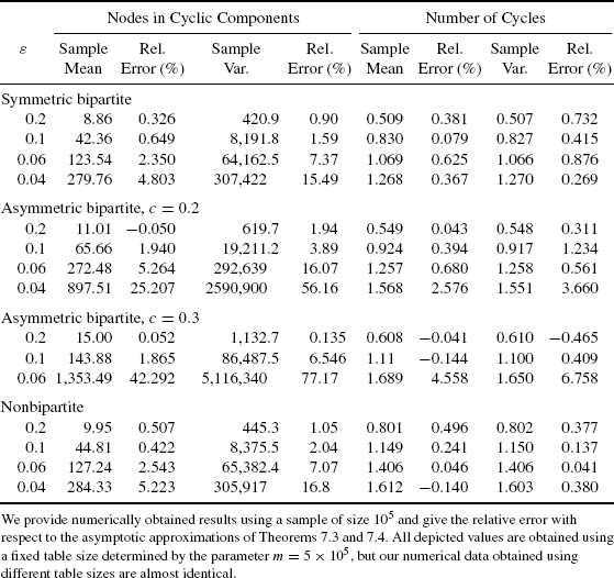
Finally, we draw our attention on the structure of cyclic components. Note that the symmetric bipartite and the ordinary model are again in some sense very similar, but not identical. Table 7.7 provides numerical data for the number of nodes in cyclic components and the number of cycles. Our experiments, using settings from m = 5 × 10³ up to m = 5 × 10⁵, show that the size of the graph does not have significant influence on this parameters. Because of this, we do not provide data for different sizes. From the results presented in Table 7.7, we see again that the asymptotic results of Theorems 7.2.3 and 7.2.4 provide suitable estimates. We notice that asymmetry leads to an increased number of cycles, and nodes in cyclic components. Furthermore, both parameters are higher if we consider the ordinary model instead of the symmetric bipartite version.

Table 7.7 The Table Shows Sample Mean and Sample Variance of the Number of Nodes Contained in Cyclic Components and the Number of Cycles.