9
Experiments Involving Formulation and Process Variables

“Design Space - The multidimensional combination and interaction of input variables (e.g., material attributes) and process parameters that have been demonstrated to provide assurance of quality”.

International Commission on Harmony for Pharmaceutical Industry Q8 (ICH 2015)

Overview

We have provided strategies, methods, and tools for experimenting with formulations. However, in many applications, there are process variables that affect the formulation and may in fact interact with the components. For example, the best baking time and temperature for bread may depend on the ingredient mix. In this chapter we provide strategies for development of formulation systems involving process variables, including design and analysis. We also present recently published research involving non-linear models that can reduce experimental efforts by as much as 50%.

CHAPTER CONTENTS

Overview

9.1 Introduction

9.2 Additive and Interactive Models

9.3 Designs for Formulations with Process Variables

9.4 The Option of Non-Linear Models

9.5 A Recommended Strategy

9.6 An Illustration Using the Fish Patty Data

9.7 Summary and Looking Forward

9.8 References

9.1 Introduction

Thus far, we have focused on experimentation and models involving only the components of formulation systems. In many applications, however, it is not just the formulation that affects the final response, but also process variables. Process variables are the additional variables that are not subject to the constraint that they must sum to 1.0. For example, in producing a blended wine the final taste and other important characteristics depend not only on the proportions of the grape varietals used, but also on process variables, such as types and amounts of fertilizers used, weather conditions of the growing season, when the grapes were harvested, temperatures at various stages of the fermentation process, type of aging barrels used, and so on.

In some cases, the mixture components and process variables do not interact. In the wine example, this would mean that the fermentation and other processing could be optimized without consideration of what grape varietals were used. This scenario would lead to the use of separate experimental designs and additive models that are a combination of a mixture model and a process variable model. In other cases, this additive scenario will not apply because the best processing conditions might depend on the varietals used. In that case, there would be interaction between the mixture and the process variables. This scenario would lead to integrated designs and models that incorporate terms to account for this interaction.

The experimental designs typically used when such interaction is anticipated tend to have a large number of blends, in order to accommodate the numbers of terms in linear models incorporating interaction (Cornell 2002, 2011). Of course, if one knows from subject matter knowledge or previous experimentation what the final model form is likely be, one may apply computer-aided designs to estimate that model. We focus on the more common situation where the experimenters suspect interaction, but are not confident in specifying the final model form before running the design and obtaining the subsequent data. Our focus is therefore neither on the optimal design for a given model, nor on the optimal model for a given set of data. Rather, we focus on a strategy for attacking these types of problems, considering alternative designs, alternative models, and factoring in the need for efficiency (time and money) in addressing problems in practice.

In this sense, we suggest a statistical engineering approach (Hoerl and Snee 2010, Anderson-Cook and Lu 2012).  Our goal is a more effective and efficient approach to address applications that involve both formulation and process variables. Statistical engineering, and its role in formulation experiments, was discussed in Chapter 2.

9.2 Additive and Interactive Models

As noted above, a key consideration in situations with both formulation and process variables is the degree to which interaction between the formulation and process variables is anticipated. If we have theory or experience that suggests that the formulation and process variables do not interact with one another, then we can fit the formulation and process models separately. In other words, here is what the overall model would become:

c(x,z) = f(x) + g(z)                                                                                                       (1)

In the model, f(x) is the formulation model, g(z) is the process variable model, and c(x,z) is the integrated formulation and process model. We refer to Equation 1 as the linear additive model, in that it simply adds a formulation model to a process variable model. In this case, f(x) would be whatever model was found appropriate for the mixture components, and g(z) would be whatever model was found appropriate for the process variables.

In many situations, however, the mixture components and process variables interact. In other words, the best time and temperature to bake a cake may depend on the ingredients in the cake. A red wine is not typically served as chilled as a white wine, and so on. In these cases, many authors, such as Cornell (2002, 2011) and Prescott (2004), suggest multiplying the formulation and process variable models, as opposed to adding them. In other words, to accommodate formulation-process interaction, we may use the following model:

c(x,z) = f(x)*g(z)                                                                                                          (2)

This multiplicative model is not linear in the parameters. Hence, the least squares solution cannot be obtained in closed form or by standard linear regression software. One approach to address this problem is to multiply out the individual terms in f(x)*g(z). Consider the case with three formulation components and two process variables. For simplicity, assume that we know these models are of the following form:

f(x) = b₁x₁ + b₂x₂ + b₃x₃ + b₁₂x₁x₂ + b₁₃x₁x₃ + b₂₃x₂x₃ + b₁₂₃x₁x₂x₃, and

g(z) = a₀ + a₁z₁ + a₂z₂ + a₁₂z₁z₂

This form would be a special cubic mixture model and a factorial process variable model. Therefore, f(x) has seven terms to estimate, and g(z) has four. If we multiply each term in f(x) by each term in g(z), this would produce 28 terms in a linearized regression model. We refer to this model as linearized because Equation 2 is, in fact, a non-linear model. By multiplying out all the terms, we create a linear model in 28 terms:

c(x,z) = f(x)*g(z) = b₁x₁*a₀ + b₁x₁*a₁z₁ + b₁x₁*a₂z₂ + b₁x₁*a₁₂z₁z₂                      (3)

                              + b₂x₂*a₀ + b₂x₂*a₁z₁ + b₂x₂*a₂z₂ + b₂x₂*a₁₂z₁z₂

                              + .............+ b₁₂₃x₁x₂x₃*a₁₂z₁z₂

Note that Equation 3 is linear in the parameters if we consider b₁a₀ to be one parameter, b₁a₁ to be another, and so on. Equation 3 can therefore be estimated with standard linear regression software, as can Equation 1. Of course, when the least squares estimates are obtained, the estimated parameter for x₁, listed as b₁a₀ in Equation 3, will in general not equal the estimated coefficient for x₁ in f(x) from Equation 2 (â₁) times the estimated intercept in g(z) from Equation 2 (ê₀). That is, if these individual terms are estimated directly from non-linear least squares, their product will not equal the estimate of b₁a₀ from Equation 3. Therefore, the least squares estimates from Equation 3 cannot be used to determine the non-linear least squares estimates from Equation 2, or vice versa.

There are a number of practical concerns in using the linearized approach, involving Equation 3 and the designs required to estimate this model. Perhaps the most important is that the designs required to estimate all terms in Equation 3 tend to be quite large. For example, Equation 3 is based on only three formulation components and two process variables, but requires estimation of 28 terms. Such large models may or may not be necessary, depending on the nature of the formulation. However, in either case, the model becomes complicated, and likely violates the principle of parsimony. This general principle states that models should be as small and simple as possible, in order to obtain a reasonable fit. As a consequence of lack of parsimony, models such as Equation 3 are generally difficult to interpret, because of the large number of terms, especially the large number of mixture and process cross products.

Because of these concerns over the linearized model and large design required, we recommend a sequential approach, similar to the sequential approach discussed in Chapter 2 for formulation problems involving no process variables. Before presenting this strategy, which involves fractional designs and use of non-linear models, we present the standard designs and models most typically used with formulation and process variable problems.

9.3 Designs for Formulations with Process Variables

Standard designs often cross a factorial design with a mixture design. For example, Cornell’s fish patty experiment (Cornell 2002) crossed a three-component simplex design involving pure blends, a centroid, and 50-50 blends, with a 2³ factorial design (three process variables each at two levels). This design is shown in Figure 9.1; the data is listed in Table 9.1. The three components were types of fish: mullet, sheepshead, and croaker. The three process variables were frying time, oven time, and oven temperature. The fish patties were both fried and baked--hence the two time variables. The response was a measure of the patty texture.

Note that at every point of the 2³ factorial design, the full simplex design was run. Alternatively, of course, one could portray this as a full factorial design at each point of the simplex. Because the simplex design had 7 points and the factorial design 8 points, the full design was 56 points, run in random order to avoid issues with split plotting (Cornell 2002, 2011).

Figure 9.1 – Cornell’s Fish Patty Design

Table 9.1 Cornell Fish Patty Data

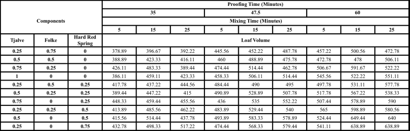
Figure 9.2 shows the crossed design run by Prescott (2004), who used a 3² process variable design (two variables each at three levels), and a 10-run simplex lattice design with three components each at four levels, for a study on baking bread. The full crossed design has 9*10 = 90 runs and is listed in Table 9.2. The components were analyzed in pseudo-component form (discussed in Chapter 6) and consist of three types of wheat: Tjalve, Folke, and Hard Red Spring. The process variables were the proofing time of the dough and mixing time, while the response was the final loaf volume.

Figure 9.2 – Prescott’s Bread Design

Table 9.2 – Prescott Bread Data

Obviously, such crossed designs can get very large very quickly. If interaction is not anticipated, however, then the designs could be much smaller. For example, in the Cornell fish patty example, there are 7*8 = 56 terms in the linearized model, which allows estimation of interaction between formulation and process variables. This requires the full 56-run crossed design just to estimate all the terms in the model and would require additional runs or replication to estimate experimental error.

Suppose, however, that interaction was not anticipated in the fish patty problem. A special cubic mixture model would have 7 terms (3 linear blending terms, three two-factor cross products, and the special cubic three-factor cross product), and a full factorial model would have 8 terms (1 intercept, 3 main effects, 3 two-factor interactions, and 1 three-factor interaction). Because the mixture model f(x) incorporates an intercept, we could drop the intercept from g(z), leaving 7 + 8 - 1 = 14 terms to estimate in a linear additive model with no interaction--i.e., c(x,z) = f(x) + g(z), per Equation 1. Clearly, a much smaller fractional design could be run or, since there is no interaction in the model, the mixture and process variables could be investigated independently.

An alternative to the full crossed design is to use a fractional design, in order to reduce the number of experimental runs. Cornell (2011) suggests the general approach of running a fractional process design at each point of the formulation design. One reason for choosing this approach, instead of a fractional formulation design at each point of the process variable design, is that the process variable designs tend to fractionate much more cleanly than do formulation designs. For the fish patty problem discussed above, Cornell (2011) noted that one option would be to run a full process variable design at the centroid of the formulation design, a half fraction of the process variable design at the pure blends, and the opposite half fraction of the process variable design at the 50-50 blends. This design is depicted in Figure 9.3. See Snee at al. (2016) for further details on generation of such designs.

Figure 9.3 – Fractional Fish Patty Design

It is important to switch the process variable design fractions between the pure blends and 50-50 blends so that all terms in g(z) can be estimated. The switching of the half fractions can be seen in Figure 9.3. Also, running a full process design at the centroid produces more data, and therefore more information, in the center of the formulation design. Note that the centroid of the formulation design is run at each of the eight points in the process design. Of course, one could run a half fraction of the process variable design at the centroid in order to reduce the size of the design or use a smaller fraction than a half fraction. The implications of fractional process variable designs are discussed in more detail in Box et al. (2005) and Montgomery (2012).

An obvious concern with this fractional design approach is to ask what might happen if there is, in fact, interaction between the process variables and formulation components? Clearly, there would not be enough data to estimate all the terms in the linearized model using the design depicted in Figure 9.3. As we shall see shortly, a sequential strategy, analogous to the strategy discussed in Chapter 2, will allow one to initially run smaller designs such as this one, while still supporting the option of larger designs that allow estimation of the full linearized model. A key aspect of this approach is the option of fitting non-linear models, which we now introduce.

9.4 The Option of Non-Linear Models

An important point to note is that Equation 2 is a model that is non-linear in the parameters. If it is directly estimated as such, as opposed to multiplying out the terms in f(x) and g(z), as in Equation 3, the number of terms to be estimated is the sum, rather than the product, of the terms in f(x) and g(z). That is, instead of Equation 3 for the sample problem with three formulation components and two process variables, we would have this:

c(x,z) = f(x)*g(z) = (b₁x₁ + b₂x₂ + b₃x₃ + b₁₂x₁x₂ + b₁₃x₁x₃ + b₂₃x₂x₃ + b₁₂₃x₁x₂x₃)*

(a₀ + a₁z₁ + a₂z₂ + a₁₂z₁z₂)                                                                          (4)

Note that in Equation 4 non-linear least squares algorithms, such as those in SAS, JMP, R, or other software or languages, would be used to directly estimate the 11 unknown parameters, b₁, b₂, and so on.

In practice, one fewer parameter than the sum of 11 is required, since Equation 4 is actually over-specified. In other words, there can be no unique least squares solution to this equation. This can be immediately seen if one considers that by multiplying f(x) by an arbitrary non-zero constant, say m, and dividing g(z) by m, the value of c(x,z) would remain unchanged. The reason is that the m and 1/m would cancel.

Since there are an infinite number of such constants m that could be multiplied by each coefficient in f(x), each producing the same residual sum of squares, there can be no unique least squares solution to Equation 4. Snee et al. (2016) addressed this over-specification by setting a₀ = 1.0, because this value for a₀ aids interpretation of the other coefficients in the model, as explained below. We follow this same approach, acknowledging that a₀ could be set to other values.

The key point, of course, is that if one can estimate Equation 4 directly as a non-linear least squares problem, there are fewer parameters to estimate, and smaller designs can be used. For example, Table 9.3 shows the number of parameters to be estimated in Cornell’s fish patty problem and Prescott’s bread problem for linearized, linear, and non-linear models. For the fish patty problem, we assume a special cubic model for f(x) and a factorial model for g(z), which is what Cornell ultimately used. For the bread formulation study, we assume a special cubic model for f(x) and a factorial model including squared terms for g(z), since this was a three-level design. Prescott started with these models but ultimately recommended a reduced model with fewer terms. The reduction in terms would be more dramatic for problems with more variables.

Table 9.3 – Number of Parameters to Be Estimated

Interpretation of individual coefficients is more complicated in these non-linear models. For example, in the simplistic case with two mixture variables and one process variable, we have the following equation:

c(x,z) = (b₁x₁ + b₂x₂ + b₁₂x₁x₂)*(a₀ + a₁z)                                                 (5)

As noted above, we can consider Equation 5 as a non-linear equation with five coefficients and use non-linear least squares to find a solution. In practice we only have four coefficients to estimate because we set a₀ = 1, for the reasons discussed previously. Using some other non-zero value for a₀ would not change model metrics, such as adjusted R², standard error, and so on. Of course, with non-linear least squares, no unique solution is guaranteed.

After estimating the terms in the non-linear model in Equation 5, we are free to multiply out the estimated terms to aid interpretation. Note that this produces a very different model from that obtained by multiplying out the terms prior to estimating the coefficients, which would produce the linearized model. After we multiply out the estimated terms in the non-linear approach to Equation 5 we obtain this equation:

$$\widehat{y}={\widehat{b}}_1{\text{x}}_1+{\widehat{b}}_2{\text{x}}_2+{\widehat{b}}_{12}{\text{x}}_1{\text{x}}_2{)}^{*}(1+{\widehat{a}}_1\text{z)=(}{\widehat{b}}_1{\text{x}}_1+{\widehat{b}}_2{\text{x}}_2+{\widehat{b}}_{12}{\text{x}}_1{\text{x}}_2)+{({\widehat{b}}_1{\text{x}}_1+{\widehat{b}}_2{\text{x}}_2+{\widehat{b}}_{12}{\text{x}}_{12}{\text{x}}_1{\text{x}}_3)}^{*}{\widehat{a}}_1\text{z}\text{(6)}$$

Equation 6 reveals why setting a₀ = 1 simplifies interpretation, as the first term is simply f(x), the formulation model. Without loss of generality we may further assume that z is scaled to have a mean of 0. Therefore, when z is at its mean value, Equation 6 simplifies to just the left part, which is the pure formulation model, f(x). Therefore, we can interpret the formulation coefficients as the blending that we estimate at the midpoint of the process variable or, alternatively, as the average blending across the entire design. This interpretation holds whether or not there is interaction with z. The interpretation of â₁ is more complicated. Note that the only place z appears in Equation 6 is through a set of interactions.

This limitation in modeling z implies the inability of the non-linear model to estimate the main effect of z uniquely from the interactions of z with the formulation variables. Why is this so? It is because the only coefficient available to incorporate the main effect of z and also its interactions with the x_i is â₁. While f(x) could be rewritten as a slack variable model with an intercept, we would still have only one degree of freedom to incorporate both the main effect of z and its interactions with the mixture variables. We view this as a drawback of the non-linear approach and speculate that the practical result will be difficulty in fitting surfaces with both large process variable main effects as well as severe interaction between mixture and process variables.

We can extend this interpretation to larger non-linear models, such as the seven-term special cubic mixture model and eight-term process variable model from the fish patty experiment. If we estimate c(x,z) = f(x)*g(z) directly as a non-linear model, we would estimate 7 + 8 – 1 = 14 coefficients. Recall that we set a₀ = 1. After solving for these 14 coefficients using non-linear least squares, we can then multiply out terms to aid interpretation. Doing so produces the following:

$$\widehat{f}{(\text{x})}^{*}(1+{\widehat{a}}_1{\text{z}}_1+{\widehat{a}}_2{\widehat{\text{z}}}_2+{\widehat{a}}_3{\widehat{\text{z}}}_3+{\widehat{a}}_{12}{\widehat{\text{z}}}_1{\widehat{\text{z}}}_2+{\widehat{a}}_{13}{\widehat{\text{z}}}_1{\widehat{\text{z}}}_3+{\widehat{a}}_{23}{\widehat{\text{z}}}_2{\widehat{\text{z}}}_3+{\widehat{a}}_{123}{\widehat{\text{z}}}_1{\widehat{\text{z}}}_2{\widehat{\text{z}}}_3)$$

Thus, the model is 1 times $\widehat{f}(\text{x})$, plus â₁z₁ times $\widehat{f}(\text{x})$, plus â₂z₂ times $\widehat{f}(\text{x})$, and so on. In other words, all other terms in the model besides $\widehat{f}(\text{x})$(x)*1 involve â_i times one or more z_i, times $\widehat{f}(\text{x})$.

Therefore, none of the main effects of the z_i can be estimated uniquely from the interaction of that z_i with the mixture variables (and their cross products), analogous to the situation in Equation 6. Similarly, interactions between the z_i, such as z₁z₂, for example, cannot be estimated uniquely from the interactions between this term and the mixture terms.

From a practical point of view, inability to estimate individual coefficients--for z₁ and x₁z₁, for example--is of greater concern than inability to estimate individual coefficients for the interactions such as z₁z₂z₃ and x₁x₂x₃z₁z₂z₃, in the sense of resolution of the design (Box et al. 2005). That is, practitioners would rarely be concerned about the practical importance of a six-factor interaction. See Snee et al. (2016) for further discussion of interpretation of the coefficients in these non-linear models.

This illustration reveals that while use of non-linear models allows much smaller designs, they also come with some disadvantages. Beyond the limitation noted above, with fewer parameters in the models, they are not as flexible as the linearized interactive models, in terms of accommodating non-linear blending. In addition, the underlying theory of non-linear models is not as well developed as for linear models, relative to such things as hypothesis testing on the model coefficients, confidence and prediction intervals, and so on. See Chapter 12 of Montgomery et al. (2012) for more detailed background on the theory of non-linear models. Therefore, we do not specifically recommend non-linear model, but rather incorporate them in an overall strategy, or plan of attack, for formulation and process variable problems.

JMP offers two different options for fitting non-linear models, which in JMP 13 are both found in the Specialized Modeling platform. Fit Curve contains several common non-linear models as built-in functions, such as the Michaelis Menten kinetic model. For a more general approach, the JMP Nonlinear platform allows users to define their own non-linear models. This is done by creating a new column, selecting the Formula option under Column Properties, and then defining the formula to be the desired non-linear function of the input variables. Users need to create the non-linear parameters used in the formula in JMP and give them initial or starting values. This latter approach using Nonlinear is the approach used below in the non-linear examples.

9.5 A Recommended Strategy

As with most experimental efforts, the choice of design and choice of model go hand-in-hand with mixture problems that have process variables. That is, the models we can estimate are determined by the design, and the appropriate design depends on the models we wish to estimate. Further, if we had a good idea of the model in advance, we could construct an optimal computer-aided design to estimate that model. However, in many practical situations our subject matter knowledge is limited, and we are not confident of the final model.

The key question is such situations is how to best approach the problem when we anticipate interaction between the mixture and process variables, but are not sure. We note that this is a very different question from asking what the optimal design is for a given model, and also different from asking what the optimal model is to fit a given set of data.

We argue that this strategy question is a statistical engineering problem, because we require an overall approach incorporating both design and analysis, perhaps in a sequential manner, in order to obtain better results. Integration of multiple tools is key. In this case, “better results” may be based on statistical criteria, or based on saving experimental effort, including time and money, or both. In other words, it may be based on finding the best business solution, as opposed to finding the best statistical solution.

We further argue that there is significant potential for savings, with minimal downside, by considering linear additive and non-linear models as options, at least early in the experimental effort. This enables use of the smaller fractional hybrid designs initially. If these smaller designs and models do not provide sufficient accuracy, then additional experimentation can be performed in a sequential manner. In this way, the best-case scenario is to reduce the experimental effect required to solve the problem by up to 50%, while the worst-case scenario is that we eventually have to run all the experimentation that a typical linearized interactive model would require. This overall strategy is illustrated in Figure 9.4, which is based on Snee at al. (2016).

Figure 9.4 – Recommended Strategy for Mixture-Process Problems

By running a fractional design initially, there is the potential to significantly reduce the amount of experimentation required to fit an adequate model. We suggest fitting both the linear additive and non-linear models to the fractional data. If the non-linear model fits appreciably better, this would indicate noteworthy interaction between the mixture and process variables. Of course, there is no guarantee that either the linear additive or non-linear model will fit well. In particular, with high degrees of interaction between mixture and process variables, linearized models will likely be needed. In some cases, a full linearized model may be estimable using the fractional design.

If experimenters are not satisfied with the models generated from the fractional design, they can run the other fraction, the fraction not run initially, to complete the full design. We feel that this option should be part of the strategy adopted at the beginning of the study. This approach would enable estimation of the full linearized model. One degree of freedom would be required to effectively block the design over time, between the first fraction and second fraction. Otherwise, there is no real disadvantage to this approach, assuming it is possible to experiment sequentially.

The model adequacy step in Figure 9.4 is meant to include a complete evaluation of model adequacy, including careful scrutiny of residuals, evaluation of potential outliers, comparison with current domain knowledge about this problem, and so on. Such evaluation of the linearized model is assumed. Hence, we have not included this as another step in Figure 9.4. Our goal in this figure is to show how to evaluate the different models in a sequential fashion, as opposed to describing the details of sound statistical model building. The latter is discussed in Box et al. (2005), for example.

9.6 An Illustration Using the Fish Patty Data

As noted previously, Cornell (2011) ran a 56-run experimental design in order to fit the linearized model involving a seven-term formulation model crossed with an eight-term process model. With 56 terms in the final model and 56 runs, there are obviously no degrees of freedom remaining to estimate experimental error. This makes it difficult to determine the adequacy of the fit, since all residuals are zero. A stepwise regression could be run to find a subset of the candidate variables and would produce an estimate of experimental error. However, Cornell did not publish such an analysis, and there are dangers associated with running automated algorithms when the number of parameters equals or exceeds the number of data points. These are beyond the scope of this book, but are discussed in Montgomery et al. (2012).

A logical question to ask is whether 56 runs are actually necessary to fit the fish patty data adequately. Recall that the non-linear model requires estimation of only 14 terms. Might a 14-term model provide an adequate fit for this study, even with far fewer than 56 runs? Following the strategy in Figure 9.4, Snee et al. (2016) fit the linear additive and also non-linear model (Equation 2) to the fractional design shown in Figure 9.3, which consists of 32 data points. As can be seen in the last two columns in Table 9.4, the non-linear model fit the fractional data better than the linear model (RMSE of 0.16 versus 0.27 for the linear model). This implies significant interaction between f(x) and g(z)--i.e., between the formulation components and process variables. Of course, in other applications the linear additive might prove to be the more useful model. We return to the other entries in Table 9.4 shortly.

Table 9.4 – Fits to Full and Fractional Fish Patty Data

	Full Data: Linearized	Full Data: Linear	Full Data Non-Linear	Factional Design: Linear	Fractional Design: Non-Linear
RMSE	0.17*	0.24	0.16	0.27	0.16
RMSE of Prediction	NA	NA	NA	0.25	0.22
Sample Data Size	56	56	56	32	32
Prediction Data Size	0	0	0	24	24
*Estimated using Lenth's Method due to zero degrees of freedom left to estimate error

The JMP output for the non-linear model is given in Table 9.5. Recall that this model was fit using the Nonlinear option under Specialized Modeling in JMP 13. In earlier versions of JMP, Nonlinear is found under the Model platform. Note that the parameter a₀ is set equal to 1.0. Fixing parameters is a possibility when running Nonlinear. Note also that JMP output from non-linear models looks very different from the output from standard linear models. Table 9.5 shows that many of the cross-product terms, both in f(x) and g(z), do not appear to be important. That is, their t ratios, obtained by dividing the estimated coefficients by their estimated standard errors, would be less than 2.0 in absolute value. There is clear non-linear blending involving x₁, based on the large t ratios for the coefficients for x₁x₂ and x₁x₃. However, none of the other cross products appear to be important; at least, none has a t ratio greater than 2.0. We return to this point shortly.

Table 9.5 – JMP Non-Linear Output: Fractional Fish Patty Data

As shown in Table 9.4, the root mean square error (RMSE) of this non-linear model is 0.16. This is hard to compare to the full 56-term linearized model because of the lack of any degrees of freedom for error in the linearized model, noted above. In such situations, one can employ Lenth’s method (Lenth 1989), which essentially identifies a subset of important terms, drops the remaining terms, and then uses the degrees of freedom from these dropped terms to estimate a pseudo or approximate RMSE. In this case, Lenth’s method produces a pseudo RMSE of 0.17, which is shown in the first column of Table 9.4. That is, the non-linear model produces a lower RMSE on this fraction of the data, using only 14 terms, than the full linearized model produces using a 56-term model initially, using all of the data.

Of course, there are limitations with such comparisons. Hence, we do not draw definitive conclusions from this one example. First of all, the RMSE from the full model is a pseudo or approximate RMSE, as noted. Further, fitting sample data in hand is always easier than predicting future data, which was not used to develop or train the model. Therefore, fitting sample data well does not guarantee good predictions of future data. In this case, the 32-run fractional design leaves a natural set of 24 additional runs that were not used to fit the model and therefore could be used to evaluate predictive accuracy.

At the bottom of Table 9.5 we see that JMP has calculated a RMSE of prediction of 0.22, rounding off to two decimal places. That is, if the model fit to the 32 data points is used to predict the other 24 data points in the full fish patty data set, these values are predicted with a RMSE of 0.22. This is, of course, higher than the 0.16 RMSE fitting the original 32 data points. As is typical, the model fit the original data set better than it predicted a hold-out data set. Therefore, while the results are promising relative to the potential of the non-linear model, we should not try to derive definitive conclusions from this one example.

If experimenters were using the recommended sequential strategy, then at this point they would need to decide whether the fractional design produced an adequate non-linear model, or whether further experimentation should be conducted to enable estimation of the full linearized model. Given that most cross-product terms in the model shown in Table 9.5 were relatively insignificant, and that the prediction RMSE was much worse than the RMSE from the original model, we might consider dropping most of the cross products and rerunning the model. Table 9.6 shows the JMP output from this model. Note that all cross products other than x₁x₂ and x₁x₃ have been set to zero, and a₀ is again set to 1.0. The RMSE for this reduced model is 0.17, rounded to two decimal places, a little larger than for the original non-linear model.

Table 9.6 – JMP Reduced Non-Linear Fish Patty Output

Note that all terms in this reduced model have t ratios greater than 2.0 in absolute value, except for the z₃ coefficient, which is almost 2.0. We can also see that the prediction RMSE is now 0.16, nearly the same as the RMSE for the data used to fit the model. This is a good sign, and it provides some evidence that this reduced model is an improvement. Keep in mind, however, that in practice experimenters would not have these additional 24 runs with which to calculate a prediction RMSE. However, if they ran additional experiments to confirm this model, as is good statistical practice, it appears that they would observe good results in terms of accuracy.

We suspect that most experimenters would be satisfied with the non-linear model from the fractional design and, following the process in Figure 9.4, would use this model to determine the next steps in the fish patty study. Per Cornell (2011), one key objective of the study was to find textures in the range of 2.0 to 3.5. Based not only upon the model shown in Table 9.6, but also the original data given in Table 9.1, this objective has been accomplished. Next, perhaps cost or other key outputs could be considered, within the ranges of these variables required to meet the texture response. We discuss multiple responses in more detail in Chapter 10. Alternatively, other process variables might be introduced. In general, there is always room for further improvement.

Conversely, should the experimenters not be satisfied with the non-linear model fit to the fractional 32-run design, they could simply run the remaining 24 points from the full design listed in Table 9.1—i.e., those formulations not run in the fractional design. With the full 56 runs available, the experimenters would then be able to run the 56-term linearized model, in addition to rerunning the linear and non-linear models with the full 56 data points. Results from these full models are also given in Table 9.4 and again show that the non-linear model fits the full data set better than the linear model, and it fits roughly equivalently to the linearized model.

9.7 Summary and Looking Forward

Many formulation experiments involve not only the formulation components, but also process variables that are not subject to the formulation constraint. This significantly complicates the experimentation and modeling of formulations. Fortunately, running hybrid designs, crossing a formulation design with a standard factorial process design, generally suffices. When these hybrid designs become impractical because of the number of experimental runs required, fractional designs can be used.

We have presented a strategy for addressing these formulation and process variable problems that begins with fractional designs, considering linear additive models and non-linear models. Both of these model types require significantly fewer parameters than the full linearized design, which crosses all terms in the formulation model, f(x) with all terms in the process variable model, g(z). The number of parameters required for the full linearized model equals those required for f(x) times those required for g(z). For the linear additive and non-linear models, the number of required parameters is the number required for f(x) plus those required for g(z), minus 1. As shown in Table 9.3, this difference is dramatic, even for relative small numbers of variables.

Should the linear additive and non-linear models prove insufficient, addition experimental runs can be made, such as running the fraction originally left out of the crossed design. With the additional experimental runs, the linearized interactive model can generally be estimated. Such a sequential approach, based on the principles of statistical engineering, provides the opportunity for significant cost savings, while providing for the larger design if it is ultimately needed. Therefore, there is much to gain and little to lose when using this strategy.

Further, we note that there is potential for further improvement in this strategy by considering computer-aided approaches to experimental design, based on the non-linear model. Computer-aided designs were discussed in Chapters 6-8, and in theory could be used to obtain optimal designs for the non-linear models presented in this chapter. There are some complications involved, such as the need for reasonable starting estimates of the non-linear parameters. Hence, this is a topic for future research at this point.

In the following chapter, we consider additional and advanced topics that can complicate formulation experiments, including multiple responses and multicollinearity.

9.8 References

Anderson-Cook, C.M., and Lu, L. (2012) “Special Issue on Statistical Engineering.” Quality Engineering, 24 (2), April-June.

Box, G.E.P., Hunter, J.S., and Hunter, W.G. (2005) Statistics for Experimenters: Design, Innovation, and Discovery, 2^nd Edition, Wiley-Interscience, Hoboken, NJ.

Cornell, J.A. (2002) Experiments with Mixtures: Designs, Models, and the Analysis of Mixture Data, 3^rd Edition, John Wiley & Sons, New York, NY.

Cornell, J.A. (2011) A Primer on Experiments with Mixtures, John Wiley & Sons, Hoboken, NJ.

Hoerl, R.W. and Snee, R.D. (2010) “Moving the Statistics Profession Forward to the Next Level.” The American Statistician, 64 (1), 10-14.

ICH, (2105), ICH Guideline Q8 (R2) on Pharmaceutical Development, EMA/CHMP/ICH/167068/2004, p. 10 (of 24). Available at: http://www.ema.europa.eu/docs/en_GB/document_library/Scientific_guideline/2009/09/WC500002872.pdf

Lenth, R.V. (1989) “Quick and Easy Analysis of Unreplicated Factorials.” Technometrics, 31(4), 469-473.

Montgomery, D. C. (2012) Design and Analysis of Experiments, 8^th Edition, John Wiley & Sons, Hoboken, NJ.

Montgomery, D.C., Peck, E.A., and Vining, G.G. (2012) Introduction to Linear Regression Analysis. 5^th Edition, John Wiley & Sons, Hoboken, NJ.

Prescott, P. (2004) "Modelling in Mixture Experiments Including Interactions With Process Variables." Quality Technology & Quantitative Management, 1(1), 87-103.

Snee, R. D., R. W. Hoerl and G. Bucci. (2016) “A Statistical Engineering Strategy for Mixture Problems with Process Variables.” Quality Engineering, 28 (3), 263-279.