
10
Additional and Advanced Topics
“Everything should be made as simple as possible, but not simpler.”
Albert Einstein
Overview
In previous chapters we have presented the primary topics and techniques needed for success in experimenting with formulations. However, in order to be fully prepared for formulation studies there are a few additional topics, such as methods for model simplification, that are helpful to know about. Some of these techniques--handling multiple responses and more complex model forms, for example--are more technically advanced; hence, we have deferred discussing them until now.
CHAPTER CONTENTS
10.2 More Advanced Model Forms
Common Alternative Model Forms
Application of Alternative Models to the Flare Data
10.4 Handling Multiple Responses
The Derringer and Suich Approach
10.5 Multicollinearity in Formulation Models
The Impact of Multicollinearity
10.1 Model Simplification
Parsimony-- keeping things as simple as possible--is a key principle in statistics, as it is applied to formulation development. There are, fortunately, many situations in which we can restate the model in a simpler form, while still maintaining its accuracy. An obvious example would be in eliminating higher order terms, such as cubic terms, if critical evaluation of the model indicates that these terms are not contributing significantly to the model. A model with only linear and quadratic terms will be simpler and, based on the model evaluation, will be equally or even more accurate in predicting future values. Recall that we do not delete components from the model without careful consideration because this affects the constraint that the formulation must sum to 1.0.
Here are some common approaches to model simplification, beyond elimination of higher order terms that are not beneficial to the model:
• Using a slack variable model
• Combining components with roughly equal effects
• Fixing components with minimal effects
• Dropping components from the model--after careful consideration
As discussed in Chapter 4, a slack variable model is one in which one component is consciously excluded from the model. In essence, it “takes up the slack” left from the other variables. This approach typically makes sense when there is one major ingredient that is either inert or has minimal direct impact on the formulation.
Consider making your favorite lemonade drink from scratch. You will need to decide how much lemon juice and sugar to use, as well as any other flavorings you might want to add. However, the bulk of the lemonade will be made up of water. Of course, water per se does not directly affect the taste of the lemonade; rather, it is the amount of sugar and lemon juice that is important. While adding more water would dilute the lemonade, this would be equivalent to reducing the lemon juice and sugar, both of which provide the taste. In cases such as this, it might make sense to use the following model:
E(y) = b0 + b1x1 + b2x2
Here are the terms of the model:
y is a measurement of taste of the lemonade
x1 is the amount of lemon juice for a fixed volume of lemonade
x2 is the amount of sugar for a fixed volume of lemonade
Of course, other models, such as a quadratic model or one with interaction, could be used to account for non-linear blending. Note that this model does not incorporate a term for water, and note also that it includes a constant, or intercept term, b0. This model form suggests that water is not critical to the taste--it merely takes up the slack from sugar and lemon juice. We can, in fact, vary sugar and lemon juice independently from one another. For quadratic or higher order terms, we could include all quadratic or higher order terms that are appropriate for non-constrained--i.e., process--variables. For example, here is the Scheffé quadratic model for three formulation variables:
E(y) = b1x1 + b2x2 + b3x3 + b12x1x2 + b13x1x3 + b23x2x3
Since we can write x3 as (1–x1–x2), it can be shown that we can alternatively write the two quadratic terms involving x3 as terms involving x1x2, x12, and x22. Therefore, here is the slack variable version of this model:
E(y) = b0 + b1x1 + b2x2 + b12x1x2 + b11x12 + b22x22
Note that both models have six terms. Scheffé special cubic models do not include all cubic terms, however. Hence, the situation with that particular model is more complicated. With linear and quadratic models, the slack variable model will give the same predictions as the corresponding formulation model; that is, at a model level they are equivalent.
A key point to keep in mind, however, is that the interpretation of slack variable model coefficients is quite different from the interpretation of formulation model coefficients. A coefficient in a slack variable model, say b1 for lemon juice here, is measuring the impact on taste of increasing the lemon juice content, while decreasing water, the slack variable, by an equal amount. Conversely, we learned in Chapter 4 that to properly interpret a linear formulation coefficient we have to compare it to the other coefficients, typically by calculating the effect. The effect measures the impact of increasing this component while simultaneously reducing the other components in equal proportions. Therefore, although slack variable models overall are equivalent to corresponding Scheffé models in terms of prediction, the coefficients are not equivalent.
Other model simplification approaches include combining ingredients, dropping ingredients from the formulation, or fixing ingredients at a specific level. Consider the situation where two or more components have roughly the same effects in a model. For example, we might have three catalysts in a linear Scheffé model in a chemistry formulation and find that the three coefficients are roughly equal. Consider the following, where x1, x2, and x3 are the three catalysts, and x4, x5, and x6 are different polymers or other components:
E(y) = 14.3x1 + 15.2x2 + 15.4x3 + 47x4 + 6.4x5 + 32x6
Note that the three catalysts have approximately the same effect on the response. Therefore, we could simplify the model by considering a new variable and call it x7, which is equal to the sum of the three catalysts. That is, x7 = x1 + x2 + x3, which represents the total amount of catalyst. Note that x7 does not need to equal 1.0, since the catalysts are only part of the formulation. In this case, here is a more parsimonious model where we would expect b7 to be approximately 15.
E(y) = b4x4 + b5x5 + b6x6 + b7x7
Recall the 10-component motor octane study discussed in Chapter 5. In this screening experiment, two sets of variables had similar effects: LH Cat Cracked A and LH Cat Cracked B had similar negative effects (-2.7, -2.6), while LL Cat Cracked and LHCC had similar positive effects (2.6, 2.9). Based on this result, it might make sense to combine each of these pairs into two new variables, thereby going from four to two variables, and reducing the total number of components from 10 to 8, an easier number to work with.
In this same octane study, there were two components that had negligible effects--that is, effects that were neither statistically significant nor practically important (HHCC A and HHCC B). Obviously, these components are not critical to the response, and they do not need to be included in the final model. However, simply eliminating them would change the formulation constraint, since the remaining components would no longer sum to 1.0. Going forward, we would probably eliminate these components from any further experimentation and modeling. When modeling the current data, we could re-express the proportions of the remaining components on the basis of all components except HHCC A and HHCC B. So measured, the sum of the remaining components would be 1.0, leaving HHCC A and HHCC B out of the model.
Similarly, if some level of such insignificant components were needed for legal, safety, cost, or some other reason, we would likely fix the level of these variables and not consider them as part of the model. For example, suppose in our lemonade example we need to incorporate an additive that has no impact on the main response of taste, but that is needed to prevent spoilage. When modeling taste, we could fix the level of the spoilage additive and measure water, lemon juice, and sugar as a proportion of the remaining formulation--that is, as a proportion of the lemonade minus the spoilage additive, analogous to the octane example. Letting x1 represent lemon juice, x2 sugar, x3 water, and x4 spoilage additive, we would redefine the components as follows:
x1* = x1/(x1 + x2 +x3)
We would define x2* and x3* similarly. These new variables would sum to 1.0, eliminating the need for a spoilage variable in our taste model.
10.2 More Advanced Model Forms
In much of the previous discussion, we have focused on Scheffé polynomial models. This is because these are probably the most commonly used models in practice. However, as with any model form, there will be applications where it is not appropriate, or where other forms are preferable. In this section we discuss some of the other model forms that are perhaps more advanced, but also useful in applications.
The first step in using such models is to detect that standard approaches, such as Scheffé polynomials, will not suffice. Consistent with the principle of parsimony, we prefer to use the simplest model form that is adequate for our purposes. Recall that in Chapter 4 we noted the importance of critical evaluation of any model as part of the overall modeling process. This included summary statistics, such as adjusted R2, and also residual analysis. In Chapter 6 we showed how the lack-of-fit test provides a formal hypothesis test on model adequacy when we have replication. When these diagnostics indicate an inadequate fit to the data-- particularly in terms of unexplained curvature--then an alternative model form is worth considering. The same would be true when efforts to address these issues--perhaps through transformations--are unsuccessful. Underlying subject matter theory may also suggest alternative model forms.
Common Alternative Model Forms
There are, of course, a large number of potential alternative forms for formulation models. We focus on some of the most common models applied in practice. One of these is based on ratios of components, rather than polynomials. A common approach is the one devised by Hackler et al. (1956). Using this approach, we take ratios of components and then treat these new variables as independent (non-formulation) variables because they no longer sum to 1.0. For a three-component system with x1, x2, and x3, for example, we might create any of the following three sets of new variables, which we refer to as z1 and z2, as shown in Table 10.1.
Table 10.1 – Examples of Ratio Model Variables
| Model | Z1 | Z2 |
| R1 | x1/(x2 + x3) | x2/x3 |
| R2 | x2/(x1 + x3) | x1/x3 |
| R3 | x3/(x1 + x2) | x1/x2 |
Each row of Table 10.1, labeled R1, R2, and R3, respectively, represents a different set of ratio variables. That is, this table provides three alternative modeling approaches, each of which is a ratio model. Note that while we had three components, we are left with only two ratio variables. Because these ratio variables, z1 and z2, are not subject to the formulation constraint, we would use standard non-formulation models. For example, we might consider the following model:
E(y) = b0 + b1z1 + b2z2 + b12z1z2 + b11z12 + b22z22
This model would be a full quadratic model in z1 and z2. In practice, experimenters would typically evaluate the different model forms, R1, R2, and R3, to determine which might provide a more accurate model for the given data set. As noted above, these models tend to provide advantages in modeling severe curvature, relative to Scheffé polynomials. Hence, this is when they could be expected to provide noteworthy improvement.
Interpretation of the coefficients in the ratio models listed above is somewhat complex. This is not only because we have a quadratic model. Even in a linear model involving only z1 and z2, the interpretation of b1, the coefficient for z1 (the ratio of x1 with x2 + x3), assumes that z2, the ratio of x2 with x3, is held constant. Snee (1973) and Cornell (2002) provide further details on construction and interpretation of ratio models, including construction of ratio models with more than three components. Below we compare several alternative model forms using a real data set.
Another common alternative model form is proposed by Becker (1968). The so-called Becker’s models also include three completely different model forms. Each uses linear terms for the components, but also includes terms often based on minimums or sums of components in place of the Scheffé higher order terms. For example, for a three-component system with x1, x2, and x3, we might define the following:
zij = min(xi, xj)
We would then construct what looks like a Scheffé polynomial, but replace the higher order terms in x with higher order terms in z. For example, we might consider the following model:
E(y) = b1x1 + b2x2 + b3x3 + b12z1z2 + b13z1z3 + b23z2z3 (1)
This would be a quadratic model. The model forms using such Becker z variables based on minimums are typically referred to as H1 models. Becker (1968) also suggested consideration of model forms based on the following alternative variables:
zij = xixj/(xi + xj), and zij = SQRT(xixj)
In both of these forms, typically referred to as H2 and H3, we would again use a model similar to Equation 1, with linear terms for the original components, but using the z variables from H2 or H3 in higher order terms. Note that the quadratic model in Equation 1 is one example, but in general we can use special cubic, cubic, or other models as well. Becker’s models provide a logical alternative to polynomial models when the latter provide an inadequate fit to the data, especially in terms of modeling non-linear blending.
St. John and Draper (1977) propose another alternative model form that is also commonly applied. It includes the inverses (reciprocals) of components. For example, an inverse model in three terms might be of the following form:
E(y) = b1x1 + b2x2 + b3x3 + c1(1/x1) + c2(1/x2) + c3(1/x3)
Note that this model form and Becker’s forms are still subject to the formulation constraint because they include linear terms for each of the three components. Inverse models tend to work best when there is extreme curvature that is not adequately addressed by other model forms. Note that both the ratio models and inverse models will have problems with components that have some zero values because we cannot calculate 1/0 or xi/0. Snee (1973) and St. John and Draper (1977) present practical methods for addressing this problem.
Application of Alternative Models to the Flare Data
To illustrate how these alternative models work, we apply them now to the flare data from McLean and Anderson (1966). Recall that this data set was presented in Chapter 6, where a Scheffé quadratic model was considered. The key output was illumination of the flare, and the four components consisted of magnesium, sodium nitrate, strontium nitrate, and a binder. An extreme vertices design was used because of constraints on the original components. In Table 10.2 we show the JMP output from fitting a quadratic Scheffé model. Note that JMP automatically creates pseudo-components for the linear terms. As we shall see shortly, this is due to the fact that the correlation between the components (multicollinearity) is lower when the components are expressed as pseudo-components.
Table 10.2 – Scheffé Quadratic Model for Flare Data

Recall from Chapter 4 that in general we do not want to test linear coefficients against the null hypothesis value of 0. Hence, we do not focus on the t ratios or p-values for the linear effects in Table 10.2. We can see that none of the non-linear blending terms are statistically significant, although a couple are close to being significant. The adjusted R2 is reasonable at .61. Hence, we would have expected more terms to be significant. Also, in the plots of this data from Chapter 6, it did appear that several of the components affected the response, and that curvature was present. Perhaps a different model form would provide a better fit to the data?
We first consider the ratio model R1, extended to include four components. Specifically, we define the variables:
z1 = x1/(x2 + x3 + x4), z2 = x2/(x3 + x4), and z3 = x3/x4
Next, we fit a polynomial model in z1, z2, and z3. Since the z variables are not formulation components, this is the form of the model:
E(y) = b0 + b1z1 + b2z2 + b3z3 + b12z1z2 + b13z1z3 + b23z2z3 +xs b11z12 + b22z22 + b33z32
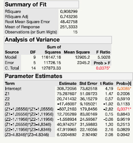
The output for this model is shown in Table 10.3. Note that the adjusted R2 has increased to 0.74, but only one of the terms in the model is statistically significant (z12).
Table 10.3 – R1 Ratio Model for Flare Data
The next model form we consider is the Becker model H3, again converted to four components. That is, we define the variables:
zij = SQRT(xixj), for i = 1 to 3 and j = i + 1 to 4
Then we fit the model:
E(y) = b1x1 + b2x2 + b3x3 + b4x4 + b12z12 + b13z13 + b14z14 + b23z23 + b24z24 + b34z34
The output for this model is given in Table 10.4. This model also fits better than the Scheffé quadratic model. With an adjusted R2 of 0.73, it is roughly the same as the R1 model. Also, we see that two of the z terms (z12 and z13) are nearly significant.
Table 10.4 – Becker H3 Model for Flare Data

Last, we consider the reciprocal models proposed by St. John and Draper (1977). These models use the standard linear terms for each component and then reciprocals for each of these as well. Here is the model we used:
E(y) = b1x1 + b2x2 + b3x3 + b4x4 + c1(1/x1) + c2(1/x2) + c3(1/x3), + c4(1/x4)
The output for this model is given in Table 10.5. Note that this model has an adjusted R2 of 0.795, better than the other models we have tried so far. Further, we have the opportunity to simplify this model, or any of the models considered, by removing insignificant terms.
Table 10.5 – Draper and St. John Model for Flare Data

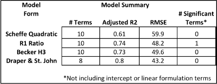
Table 10.6 compares the different models we have used on the flare data set. The St. John and Draper model (1977) appears to fit the data best, although we have not considered all versions of the ratio or Becker’s models. Additional evaluation, using the overall model building process as discussed in Chapter 4, would likely lead to an even better model. We present Table 10.6 only in order to illustrate the potential for improvement possible when we consider additional model forms. We return to the surprising last column, where only one term besides an intercept or linear formulation term is statistically significant, in our discussion of multicollinearity in Section 10.5.
Table 10.6 – Flare Model Comparison
10.3 Response Optimization
When experimenting with three components, it is relatively easy to identify the maximum or minimum predicted value within the simplex, or constrained design space. We simply plot contours of the model and look for the optimum. However,
finding the optimum when we have five, six, or more components is not trivial. We can plot only three components at a time, perhaps four with three-dimensional graphics, but these contours will depend on the fixed levels of the other components. Consider the Scheffé quadratic model for the flare experiment data, given in Table 10.2.
Figure 10.1 shows the contours of illumination for this model. These come from the JMP option Mixture Profiler, as explained in Chapter 4. Note that the graph shows a simplex involving x1, x2, and x3. However, there are four components in this design; x4 has been set equal to 0.055 by JMP. We can change the value at which x4 is fixed, or we can change which of the four components is fixed and view contours of the other three. Note that this graph also illustrates the constrained region within which we experimented.
Figure 10.1 – Contours for Scheffé Quadratic Model

Note that if there is non-linear blending, as there is in this case, then the shapes of the contours might change quite significantly if levels of the components that were excluded from the plots were modified. Clearly, we need another approach for model optimization with more than three components. Fortunately, analytical tools for model optimization are available. One method that has been effectively used for decades is quadratic programming (Nocedal and Wright 2006). It can be used to analytically optimize a quadratic function, including equations involving constraints on the variables. More general methods can be used to optimize complex functions, such as the alternative models noted above. While common software, such as Excel, often has a basic function for optimization, some of these analytical solutions require either sophisticated software, or programming on the part of the user, or perhaps both. Isn’t there a simpler approach?
Fortunately, there is. Some software programs, such as JMP, offer optimization algorithms within their regression routines. Recall from Chapter 4 that the JMP option Prediction Profiler provides graphical representation of response surfaces. One possibility within the profiler is to create a “desirability function” and then optimize it. The default for the desirability function is a linear function of the response y, which is simply 0 for the minimum observed y value and 1 at the maximum. The user can create more complex relationships between the desirability function and the response. For example, there could be a range of response values that are considered equally desirable. This function is created in JMP 13 by selecting Optimization and Desirability in Prediction Profiler and then selecting Desirability Functions.
The intent is that this function should reflect the overall desirability, or “goodness”, of the response and put it on a 0 to 1 scale. This desirability may or may not be linear, based on subject matter knowledge. For example, for some applications we may want to maximize the response, but in other cases we may want to simply hit a target, in which case having a higher predicted value is less desirable. Once a desirability function has been created, we can then optimize it using the option Maximize Desirability, also under Optimization and Desirability.
Consider the Scheffé quadratic model for the flare experiment data that is given in Table 10.2. In Figure 10.2 we show the JMP output from the Maximize and Remember Desirability option, which lists the specific optimum combinations of components. Note that the highest observed value may not correspond to the point of the highest predicted value, because of modeling error and also random variation in the response values. In this case, we see that the maximum predicted illumination occurs approximately at the point x1 = 0.52, x2 = 0.23, x3 = 0.17, and x4 = 0.08. The predicted illumination is 397. This is very close to the 14th point in the data set, which produced an observed illumination of 410, close to the predicted value of 397. JMP also gives us a confidence interval for the average illumination at this point.
Figure 10.2 – Optimization of Scheffé Quadratic Model

10.4 Handling Multiple Responses
We have noted several times that most real formulation problems involve multiple responses. For virtually all commercial applications, cost will be a response of interest, in addition to the other responses that quantify quality characteristics. In Chapter 8, we presented the Chick and Piepel (1984) data, which had three responses: temperature, spinel phase yield, and weight loss. Obviously, to produce a commercially successful pharmaceutical, chemical, plastic, or other product, all the responses must be in an acceptable range. We cannot have excellent quality but at an unacceptable price, or vice versa. How should experimenters approach such problems?
As noted previously, it is often the case that the responses, especially responses related to product quality, are correlated with one another. This means that when one response tends to be high, the others tend to also be high, or low if the correlation is negative. When this is the case, researchers can usually optimize the response that is considered primary, or most important, using the methods discussed in Section 10.3. They can then verify that the other responses are in an acceptable range at this optimum point for the primary response. In the Chick and Piepel example, the optimum regions for weight loss turned out to be desirable, or at least acceptable, for the other responses. Leesawat et al. (2004) provide another example of this approach.
Of course, the responses will not always be correlated and, even if they are, the best region for one response may be the worst region for another. For example, in food science the most expensive ingredients often produce the best tasting final product, meaning that cost and taste cannot both be optimized. When this occurs, we need another, more general approach.
One such approach, especially useful with a small number of components, is the visual comparison of contours plots of the different responses. Optimal or acceptable regions can be identified in each and then compared in an attempt to find formulations that satisfy the requirements of all responses. For example, we saw in Figure 10.1 above that illumination appeared to be maximized when x4 was fixed at 0.055, and x1 was about 0.53, x2 was about 0.23, and x3 was about 0.19. Note that the exact mathematical optimum was calculated by JMP and given at the bottom of Figure 10.2. In Figure 10.1 we were simply evaluating the graph by eye.
Suppose a second contour plot for cost of the formulation showed a minimum in the lower right of the constrained region, say around the point x1 = 0.4, x2 = 0.145, x3 = 0.35, again with x4 fixed at 0.055. This point is highlighted in Figure 10.3, which shows the illumination contours in the background. The predicted illumination for this optimal cost point is about 250, well below the theoretical maximum of 397.6. At this point, we need to make some tradeoffs between cost and illumination. Obviously, subject matter knowledge and marketing strategy would be helpful. However, with the current components under the current constraints, we cannot maximize both cost and illumination at the same time.
Figure 10.3 – Contours of Illumination with Cost Minimum Point Noted

Another approach is to create some type of desirability function, which could be a weighted average of the various responses. Using the individual models developed for each response, experimenters would plug these model outputs into the desirability function, so that a single equation could be used to quantify desirability as function of the components. For example, suppose we had three responses, y1, y2, and y3. Each of these is a function of four components, x1 – x4, but the regression equations could be quite different for each response. Let us say that these are the equations:
E(y1) = f1(x1-x4)
E(y2) = f2(x1-x4)
E(y3) = f3(x1-x4)
Further, let us suppose that after careful consideration, we have chosen the following function as an overall measure of desirability of the responses as a set:
D(y1-y3) = 4y1 + 2y2 - y3
This would imply that maximizing y1 is roughly twice as important as maximizing y2 and four times as important as minimizing y3. The fact that y3 has a minus sign implies that we would like to minimize it, rather than maximize it. This equation also assumes that the three responses are in roughly equivalent units of measurement, so some standardization might be required as a preliminary step. For example, if we subtract the sample mean and divide by the sample standard deviation of each response, then each will have a mean of zero and a standard deviation of 1. Hence, they would be in the same units.
Once we have defined the desirability function, we can insert the prediction equations for y1-y3 as follows:
D(x1-x4) = 4f1(x1-x4) + 2f2(x1-x4) - f3(x1-x4)
Note that the desirability equation is now a function of the components, rather than the responses. We could then optimize this equation to find the best overall formulation, considering all the responses. This approach of combining the separate models is generally preferred to creating an overall desirability response and fitting one model to that response. The reason is that the approach we have presented above allows us to fit specific models to each response and is therefore likely to be more accurate in predicting desirability.
The Derringer and Suich Approach
Derringer and Suich (1980) proposed a somewhat more sophisticated version of the desirability function approach that is popular in applications. They proposed a multiplicative desirability function based on individual desirability functions for each response, involving upper (Ui), target (Ti), and lower (Li) values for each response. The overall desirability function is obtained by the following:
D = (d1(y1)*d2(y2)*…dk(yk))1/k, where we have k responses
The individual desirability functions, di(yi), are set to 0 when a completely undesirable value of yi is predicted, and 1.0 when the absolute best yi is predicted. Therefore, the minimum value of D is 0, and the maximum value is 1.0. For responses to be maximized, Li would be the minimum acceptable value--i.e., a value below which the desirability function would be set to 0. Ti would be the level we would like to achieve, if possible and, because this response is to be maximized, there would be no Ui. The situation would be reversed for responses to be minimized; Ui would be the maximum allowable, Ti would be the desired level, and there would be no Li. For responses with a target value, we would let Ti be this target value, and Li and Ui would be the minimum and maximum allowable values.
The individual desirability function for a response to be maximized would then be the following:
0 if yi < Lidi(yi) = (yi−Li)/(Ti-Ti) if Li < yi < Ti 1 if yi > Ti
For a response to be minimized, we would essentially reverse di as follows:
0 if yi > Uidi(yi) = (Ui - yi)/(Ui - Ti) if Ti < yi < Ui 1 if yi < Ti
For a response intended to hit a specific target level, say Ti, as closely as possible:
0 if yi < Lidi(yi) = (yi - Li)/(Ti - Li) if Li < yi < Ti (Ui - yi)/(Ui - Ti) if Ti < yi < Ui 0 if yi > Ui
Note that the equations given above are a simplified version of the Derringer-Suich equations. The original publication suggested taking these values (those in parentheses, such as (yi - Li)/(Ti - Li) ) to a power. Use of different powers for different responses would essentially weight the responses. However, in practice these powers are often set to 1, which is the simplified version shown above.
We use the Heinsman and Montgomery (1995) household cleaner models to illustrate how the Derringer-Suich approach works in practice. Heinsman and Montgomery used four surfactants in their design, which comprise the four components, x1-x4. They also considered four responses: product life (lather), grease-cutting ability, measured in “soil loads”, foam height, a measure of the ability to produce foam, and total foam, a measure of how long the foam lasts in the presence of grease. All responses were to be maximized, although the first, lather, was considered most important. The design that was chosen was a 20-run D-optimal design that was intended to support a quadratic Scheffé model. The D-optimal design was chosen because of single component constraints, resulting in an irregularly shaped design region.
The resulting equations for the four responses were quite different from one another. Two of them involved square root transformations, two used quadratic Scheffé models, and two were Scheffé special cubic models. The response maximums did not occur in the same locations in the design space, requiring a more sophisticated approach. Heinsman and Montgomery therefore used the Derringer-Suich approach with all responses to be maximized. However, for two of the responses, y1 and y2, they set Li = Ti. In other words, they decided to force responses at or above the target value Ti. Mathematically, the maximization equation above is undefined if Li = Ti because we end up dividing by zero. Therefore, Heinsman and Montgomery set d1(y1) and d2(y2) = 0 if yi < Ti, and d1(y1) and d2(y2) = 1 if yi ≥ Ti. This decision forced a solution that met these two target values, and it is a practical way of weighting these responses higher than the others.
Heinsman and Montgomery used mathematical programming, a more general form of quadratic programming, to optimize D as a function of x1-x4. The maximum was found at x1 = 0.587, x2 = 0.377, x3 = 0.0, and x4 = 0.036. Note that the solution set x3 = 0.0, simplifying the model to three components, as we discussed in Section 10.1. The minimum values (Li), targets (Ti - where appropriate), and final predicted responses at the maximum point for D are given in Table 10.7. Note that while the target values for y1 and y2 were obtained (or exceeded), it was not possible to meet the targets for all four responses. This is typical in multi-response situations.
Table 10.7 – Results of Heinsman-Montgomery DS Optimization
| Response | Minimum | Target | Solution |
| y1 | 3.5 | NA | 3.5 |
| y2 | 19 | NA | 21.99 |
| y3 | 82 | 105 | 96 |
| y4 | 1,000 | 1,436 | 1,417 |
Li et al. (2011) provide another case study using the Derringer-Suich approach.
10.5 Multicollinearity in Formulation Models
What Is Multicollinearity?
We saw in Table 10.2 that the Scheffé quadratic model produced an adjusted R2 of 0.61 when fit to the flare data, but that none of the non-linear blending terms were statistically significant. Conversely, a linear model using only the four components produces an adjusted R2 of 0.42. It may seem odd that we are able to obtain a better fit to the data with quadratic terms, but that we can’t determine which of these terms are actually important. Recall also from Table 10.6 that only one term that was not an intercept or linear blending term, among all the alternative models considered, was statistically significant. This lack of significance for individual terms in regression models, even in models that fit the data well, is a common problem both with formulations as well as modeling in general.
One of the causes for this problem is multicollinearity, which refers to correlation among the predictor variables--component levels in this case. Correlation among the predictor variables makes it difficult to uniquely determine the effect of each variable in the model. Often, we are able to accurately predict the response within the region of interest, but are not confident as to which terms in the model are producing the fit. Hoerl and Kennard (1970) have shown that extreme multicollinearity can produce regression coefficients that are on the average too large and often have the wrong signs.
We can see the underlying reason for the problems that are associated with multicollinearity by considering a simple, hypothetical data set. We first consider multicollinearity in general-- i.e., in process variable models--and then consider the unique challenges of multicollinearity when experimenting with formulations.
Suppose we have two key process variables for a chemical reactor, which we will refer to as temperature (x1) and pressure (x2). The response of interest is the yield of the reaction. Suppose that the engineers are not trained in design of experiments and that they are trying to improve yield. They might change both temperature and pressure at the same time, producing a higher yield. This improvement might convince them to increase both temperature and pressure again, perhaps increasing yield again. Eventually, they might reach a practical maximum of temperature and pressure, beyond which they cannot go. What might the resulting data from their experimentation look like? It might look like the data in Table 10.8.
Table 10.8 – Hypothetical Yield Data
| Temperature | Pressure | Yield |
| 100 | 2 | 70 |
| 150 | 3 | 75 |
| 200 | 4 | 80 |
| 250 | 5 | 85 |
| 300 | 6 | 90 |
| 350 | 7 | 95 |
In Figure 10.4 we show a plot of temperature versus yield. Also, we have shown the level of pressure on the right scale. Upon first glance at Figure 10.4, we note that yield consistently increases as temperature increases. That is, they are perfectly correlated. Yield appears to be a function of temperature with no noise or random variation.
However, if we look at the right scale for pressure, we see that pressure is also perfectly correlated with temperature because the engineers changed both at exactly the same time. Therefore, pressure is also perfectly correlated with the yield. We can ask whether increases in yield were caused by increases in temperature, as we originally thought, or by increases in pressure, or perhaps a combination of both? Clearly, this question is impossible to answer with this data because temperature and pressure were increased at exactly the same times. Even though a linear model in either temperature or pressure would fit this yield data perfectly, with an adjusted R2 of 1.0, we cannot differentiate the unique effect of temperature from that of pressure.
Figure 10.4 – Plot of Yield versus Temperature and Pressure

Standard experimental designs for process variables, such as factorial designs, avoid the perfect correlation seen in Figure 10.4, and typically produce no or at least very low multicollinearity. In fact, one of the main motivations for designed experiments is to obtain data that does not suffer from multicollinearity. In formulation experiments, however, we have the constraint that the components sum to 1.0. Hence, it is not possible to obtain components that are totally uncorrelated. Constraints on the components almost always worsen these correlations because they often produce irregularly shaped design regions and because the coefficients represent extrapolation from our restricted design space. When we have several components and then add non-linear blending terms into the model as well, the correlation now involves multiple variables--i.e., it becomes multicollinearity, and it becomes worse. We can keep such correlation to a minimum, however, through standard formulation designs such as those based on the simplex.
Quantifying Multicollinearity
There are several ways to quantify multicollinearity and its effects on model coefficients.
Calculating individual correlation coefficients between components is not a good approach, however, for a couple of reasons. First of all, we would have to calculate a correlation coefficient for every possible pair of components. Second, there could be a source of multicollinearity involving several variables (a linear combination) that would not be obvious from individual correlations. For example, with a standard simplex-centroid design in three components, the correlation between any pair of components will be moderate--about -0.5. Yet, as we know, there is a perfect linear association between x1, x2, and x3, producing the formulation constraint. This perfect multicollinearity between the three components is what prevents us from fitting a standard regression model with three linear coefficients and also an intercept. As discussed previously, this problem is typically addressed by removing the intercept from the model.
Those with a background in linear algebra often use multicollinearity metrics associated with the ability to invert the data matrix, which is required to fit regression models. These metrics include the determinant, eigenvalues, and condition number of the matrix. A simpler approach is to calculate variance inflation factors, or VIFs, which are produced by many regression software applications, including JMP. In addition to being found in software, they are also on a scale that directly quantifies their negative impact on the model itself. This makes interpretation much easier. In the discussion below, we focus on VIFs. See Montgomery et al. (2012) for a more detailed discussion of multicollinearity, its quantification, and its effects on regression models. Snee and Rayner (1982) and
Cornell (2002) provide more focused discussions relative to multicollinearity in formulation models.
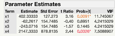
The VIF is precisely what it sounds like, a measure of the degree to which the estimated variance of individual coefficients has been inflated due to multicollinearity. That is, a VIF of 4 means that the variance of an estimated regression coefficient is four times what it would have been if no multicollinearity had been present. Let’s go back to the flare data to illustrate this point. In Table 10.9 we see the JMP output for a linear Scheffé model fit to the flare data. Note that JMP automatically transforms the linear terms by converting to pseudo-components. We discuss the reasons for this below. In this case, we have also asked for the VIFs to be given for each coefficient in the model. The VIFs are obtained by right-clicking inside the Parameter Estimates output. Another menu will appear; select Columns, and then VIFs, and the VIFs will be added to this table.
Note in Table 10.9 that the VIF for x4 is 2.19. The estimated standard error for the coefficient for x4 (b4) is 319.4. This is a measure of how much uncertainty is associated with our estimated b4, which is 989.3 in this case. Because the VIF is 2.19, we know that this estimated standard error of about 319.4 is inflated because of the multicollinearity between the four components.
Table 10.9 – VIFs for Linear Flare Model

Specifically, if the variance is 2.19 times larger than it would have been without any multicollinearity, then the standard deviation (standard error) is √2.19=1.48 times as large as it would have been. In other words, if we had components that were uncorrelated with each other, then the estimated standard error for b4 would have been 319.4/1.48 = 215.8. Each of the VIFs therefore gives us a direct measure of how inflated the variances or standard errors of the estimated coefficients are. We can quickly calculate what the standard errors would have been, had there been no multicollinearity.
So how large is too large? Marquardt and Snee (1975) recommend that VIFs over 5 be considered evidence of moderate multicollinearity, while VIFs over 10 be considered evidence of severe multicollinearity. The minimum VIF is 1.0, indicating no inflation, but there is no maximum; we have seen VIFs in the thousands, indicating very severe problems with multicollinearity. Keep in mind that VIFs refer to variances; if we take the square root of the VIF it would refer to the inflation of the standard errors themselves. Recall also that perfect VIFs of 1.0 are not possible in formulation models because of the constraint that the components must sum to 1.0. The situation with the linear flare model is therefore not bad; no VIFs are over 5.0
The Impact of Multicollinearity
Multicollinearity obviously inflates the standard errors of our regression coefficients, making it harder to uniquely determine the effect of each component. That is, our uncertainty about the population regression coefficient, bi, is greater. The estimate could be very far from the true population value--i.e., far from the “truth”, and even have the wrong sign. In severe cases, the estimated coefficient may appear to be nonsensical based on subject matter knowledge.
The inflated standard error often leads to low t ratios, and terms that are therefore not statistically significant, even if the term is actually important. Recall that the t ratio is just the estimated coefficient divided by the standard error. If the standard error is inflated, the t ratio will tend to be low. It is possible to have models with a large adjusted R2 and with high F ratios testing overall model fit, but with no terms in the model statistically significant. In other words, the model can determine that the x variables as a set are affecting the response, and perhaps predict well within our design space, but it cannot determine which specific terms are important. This was the case with the quadratic model fit to the flare data. Of course, such a situation limits the degree of insight that can be obtained from the model, as well as complicating the task of model simplification. Which model terms should be kept and which can be removed? If no terms are statistically significant, this question can be very hard to answer.
Beyond complicating model interpretation and simplification, severe multicollinearity can also cause numerical problems for regression algorithms. As the VIFs increase, the numerical problem of inverting the data matrix, which is a required step in obtaining least squares solutions, becomes more difficult. Even with modern computing capabilities, the software may not be able to accurately invert the matrix. In such cases, software programs such as JMP will often drop variables from the model in order to obtain a solution. Typically, a warning message is given to the user explaining that terms were dropped because of severe multicollinearity, in order to obtain an accurate solution. However, the model that the user originally wished to fit cannot be accurately estimated.
As noted previously, there will always be some multicollinearity in formulation models because of the constraint that the components must sum to 1.0. Also, higher order terms, such as quadratic or cubic terms, often add to the multicollinearity because x1 will not only be correlated with x2 and x3, but also to some degree with the terms x1x2, x1x3, and x1x2x3. Table 10.10 shows the VIFs from the quadratic flare model. Note that in every case the VIFs have increased from the linear model in Table 10.9. The VIF for x4 has increased from 2.19 to 1,612. Three of the quadratic terms have VIFs in the hundreds. We have gone from a fairly good situation with the linear model to extremely high multicollinearity with the quadratic, as shown in Table 10.10.
Table 10.10 – VIFs for Quadratic Flare Model

The key implication of Table 10.10 is that multicollinearity also presents a challenge to developing higher order models, in that higher order terms will likely provide a better fit to the data, but at the price of adding multicollinearity. Therefore, we must balance model accuracy with the ability to interpret and gain insight from the model. Such issues tend to be worse with constrained design spaces, because we no longer have an entire simplex, but may have a very irregular shape, limiting our flexibility in creating designs with minimal multicollinearity.
Addressing Multicollinearity
Clearly, multicollinearity causes problems in regression analysis, and it is impossible to completely avoid in formulations development. So what should we do about it, to mitigate its effects? Possible counter measures include everything from very simple precautions to much more complex methods. We will focus on the more basic steps that can be taken to make the problem manageable. The simplest approach, as one might imagine, is to avoid multicollinearity, at least to the degree possible. The standard simplex-centroid designs, with or without checkpoints, and also simplex-lattice designs are structured in such a way as to limit correlation between the components, including correlation with higher order terms. This is one of the reasons that such designs are used so often in applications.
As noted above, constrained formulation spaces often limit our ability to construct designs with minimal multicollinearity. In such cases, D-optimal designs are a common approach to selecting extreme vertices, and other candidate points in the design, as discussed in Chapters 7 and 8. Because the D-optimal criterion minimizes the size of the joint confidence interval of the regression parameters, it does take correlation among the terms into account. Multicollinearity will tend to increase the size of the joint confidence interval. Hence, the D-optimal criterion generally avoids designs with high multicollinearity, at least to the degree possible.
If we are analyzing data and detect multicollinearity--through VIFs for example--there are still simple steps we can take to alleviate the problem after the fact, at least to some degree. For example, with constrained regions, converting to pseudo-components often reduces the multicollinearity and thereby the VIFs. One reason for this is that the linear coefficients in the original variables are predicting the response at a pure blend. However, with constrained formulations, this is outside our actual design space--perhaps well outside. When we convert to pseudo-components, the pure blend is now the maximum possible value for this component--i.e., it is now within our design space. See Cornell (2002) for a more detailed explanation of why transforming to pseudo-components often works in reducing multicollinearity.
We can observe this phenomenon by returning to the flare data. As noted above, VIFs are computed in JMP by right-clicking the Parameter Table. Next, click the Columns option and then the VIF option. Table 10.11 shows the VIFs for the linear model, but in this case we have overridden the JMP default of converting to pseudo-components. Recall from Table 10.9 that when converting to pseudo-components, the VIFs were all small, below the 5.0 threshold for moderate multicollinearity. However, in Table 10.11 we see that two of the VIFs are above 5.0, and one is above 10.0, the limit for severe multicollinearity. The models are equivalent overall, in terms of adjusted R2, root mean square error, contour plots, and so on, but most of the multicollinearity was removed by a simple conversion to pseudo-components. When users list variables as formulation components (mixture in JMP), and they are constrained--not varying from 0 to 1.0--JMP automatically converts to pseudo-components for just this reason. If other software does not, users should manually convert to pseudo-components.
Table 10.11 – VIFs for Linear Flare Model: No Pseudo-components
We saw in Table 10.10 that incorporating higher order terms in formulation models can also increase multicollinearity. We might say that this design, because of the constraints, does not support the estimation of quadratic terms involving x4 well. Although we are not familiar with the chemistry of this particular application, subject matter knowledge in some chemical applications suggests that the binder primarily holds the chemicals together and therefore should blend linearly--i.e., it would be less likely to be involved in non-linear blending. Therefore, based on the VIFs and possibly subject matter knowledge, we might consider dropping the quadratic terms involving x4 from the model in order to reduce multicollinearity. Table 10.12 shows VIFs for a model with only quadratic terms for x1-x3. While not shown in the table, the adjusted R2 has increased from 0.61 to 0.69 without the quadratic terms involving x4, and the VIFs are much more reasonable. Also, all three quadratic terms are close to being statistically significant. Subject to critical model evaluation through residual analysis and confirmation from subject matter theory, we would likely prefer to use this model in practice. It fits the data better, and has much less multicollinearity.
Table 10.12 – VIFs for Reduced Quadratic Flare Model

Dropping terms from the model, especially terms with high VIFs that are not statistically significant, is therefore another strategy for reducing multicollinearity. In general, the simpler the model, the lower the multicollinearity. Therefore, the methods discussed in Section 10.1 for model simplification can also be applied to reduce multicollinearity. Another approach is to consider alternative model forms, such as those discussed in Section 10.2. Note that VIFs can be calculated on any linear model in the parameters. VIFs are not defined for non-linear models, such as those discussed in Chapter 9.
Last, estimation methods that are more complex than least squares can be applied. Ridge regression (Hoerl and Kennard 1970, Marquardt and Snee 1975) is one such approach that was specifically developed to address inflation of coefficient variances because of multicollinearity. In essence, ridge regression shrinks the size of the coefficients toward the null hypothesis values, which would be ȳ for the linear terms and 0 for higher order terms. Because of the inflated variances that are due to multicollinearity, the coefficients will tend to be too large in absolute value. See St. John (1984) and Box and Draper (2007) for more details on this approach. More recently, methods related to or involving ridge regression, such as the lasso and elastic net, have been introduced into the literature (James et al. 2013). More research is needed relative to their application to formulation data, however.
10.6 Summary
We have considered several topics that, while important, are somewhat beyond the scope of this book. We therefore provide this chapter to present additional material that we have found useful in applications. Model simplification, while not complicated in itself, is of practical importance and deserves careful consideration when building models. Similarly, the Scheffé polynomial models are effective in a wide diversity of applications involving formulations. However, no single model form is universally best. For some data sets, an alternative model form, such as one of those presented in this chapter, will provide a better fit to the data, and may make more sense from a subject matter knowledge point of view.
Optimization of the final model form can be challenging, especially with models involving significant curvature. Fortunately, both analytical techniques and commercial software designed for model optimization are readily available. JMP is one example of software that allows the user to find the best formulations. Of course, with multiple response systems the problem is more complicated because what is best for one response may not be for another. Therefore, having strategies for attacking this problem, such as the Derringer-Suich approach, can be critical to success.
Multicollinearity, correlation between the terms in a regression model, is a common problem both in formulation models and process variable models. Multicollinearity causes inflated variances for the coefficients in the model, often producing nonsensical answers, such as coefficients with the wrong signs. At a minimum, it produces large standard errors for the coefficient estimates, often resulting in insignificant t ratios, even for terms that we believe are important based on subject matter knowledge. Fortunately, simple techniques, such as conversion to pseudo-components or model simplification, can help reduce the problem. More advanced methods, such as ridge regression, can help when the simple methods are not sufficient.
We believe that the methods presented in this chapter, combined with those from previous chapters, will be practically useful to experimenters working on real problems with formulations. We wish you the best in your applications.
10.7 References
Becker, N. G. (1968) “Models for the Response of a Mixture.” Journal of the Royal Statistical Society, Series B (Methodological), 30 (2), 349-358.
Chick, L. A and G. F. Piepel. (1984) “Statistically Designed Optimization of a Glass Composition.” Journal of the American Ceramic Society, 67 (11), 763-768.
Cornell, J.A. (2002) Experiments with Mixtures: Designs, Models, and the Analysis of Mixture Data. 3rd Edition, John Wiley & Sons, New York, NY.
Derringer. G. L., and Suich, R. (1980) “Simultaneous Optimization of Several Response Variables.” Journal of Quality Technology, 12 (4), 214-219.
Draper, N. R. and St. John, R.C. (1977) “Designs in Three and Four Components with Mixtures Models With Inverse Terms.” Technometrics, 19(2), 117-130.
Hackler, W.C., Kriegel, W.W., and Hader, R.J. (1956). “Effect of Raw-Material Ratios on Absorption of Whiteware Compositions.” Journal of the American Ceramic Society, 39 (1), 20-25.
Heinsman, J.A., and Montgomery, D. C. (1995) “Optimization of a Household Product Formulation Using a Mixture Experiment.” Quality Engineering, 7(3), 583-600.
Hoerl, A.E., and Kennard, R.W. (1970) “Ridge Regression: Biased Estimation for Nonorthogonal Problems.” Technometrics, 12(1), 55-67.
James, G., Witten, D., Hastie, T., and Tibshirani, R. (2013) An Introduction to Statistical Learning: With Applications in R, Springer, New York, NY.
Leesawat, P., Laopongpaisan, A., and Sirithunyalug, J. (2004) “Optimization of Direct Compression Aspirin Tablet Using Statistical Mixture Design.” Chiang Mai University Journal of Natural Sciences, 3 (2), 97-112.
Li, W., Yi, S., Wang, Z., Chen, S., Xin, S., Xie, J., Zhao, C. (2011) “Self-nanoemulsifying Drug Delivery System of Persimmon Leaf Extract: Optimization and Bioavailability Studies.” International Journal of Pharmaceutics, 420 (1), 161-171.
Marquardt, D.W., and Snee, R.D. (1975) “Ridge Regression in Practice.” The American Statistician, 29 (1), 3-20.
McLean, R. A. and V. L. Anderson. (1966) “Extreme Vertices Design of Mixture Experiments.” Technometrics, 8 (3), 447-454.
Montgomery, D.C., Peck, E.A., and Vining, G.G. (2012) Introduction to Linear Regression Analysis. 5th Edition, John Wiley & Sons, Hoboken, NJ.
Nocedal, J., and Wright, S.J. (2006) Numerical Optimization. 2nd Edition, (2nd ed.), Springer, New York, NY.
Snee, R. D. (1973) “Techniques for the Analysis of Mixture Data.” Technometrics, 15 (3), 517-528.
Snee, R. D. and A. A. Rayner. (1982) “Assessing the Accuracy of Mixture Model Regression Calculations.” Journal of Quality Technology, 14 (2), 67-79.
St. John, R.C. (1984) “Experiments With Mixtures, Ill-Conditioning, and Ridge Regression.” Journal of Quality Technology, 16 (2), 81-96.