1 Introduction to Formulations Development

“Manufacturers would often experiment, changing their formulas after tests of a finished powder proved it was not giving the results desired”.

Norman B. Wilkinson, Explosives in History, 1966

Overview

Many products are created by mixing or blending several components or ingredients. In the statistical literature the term mixture is used to define a formulation, blend, or composition. In this chapter, we discuss some examples of formulation and how to display formulations graphically. We also present some case studies that illustrate the problems addressed in formulation studies and show how such problems are resolved.

By the end of this chapter, here is what you will have:

•   An introduction to formulations

•   An understanding of how formulations are different from other types of experimentation

•   Examples of formulations from various fields of study

CHAPTER CONTENTS

Overview

1.1 Examples of Formulations

1.2 How Formulation Experiments are Different

Displaying Formulation Compositions Using Trilinear Coordinates

1.3 Formulation Case Studies

Food Product

Pharmaceutical Tablet Formulation

Lubricant Formulation

Pharmaceutical Tablet Compactability

1.4 Summary and Looking Forward

1.5 References

1.1 Examples of Formulations

Here are some examples of well-known products that are formulated by mixing together two or more ingredients or components:

•   Pharmaceutical Tablets

•   Food

•   Gasoline Blends

•   Metal Alloys

•   Rocket Propellants

•   Aerosol Formulations

•   Paints

•   Textile Fiber Blends

•   Concrete

•   Dyes

•   Rubber

•   Cocktails

This list illustrates the variety of scientific areas in which mixture experimentation is used. Here are some details.

Pharmaceutical Tablets –The tablets that we take are formulated by mixing the active ingredient (the compound used to treat the disease) with a number of other ingredients to form and manufacture the tablet. The ingredients include diluents, disintegrates, lubricants, glidants, binders, and fillers. How well the tablet dissolves is often a function of one or more of these ingredients.

Food –A variety of foods are manufactured by mixing several ingredients. For example, the development of cake mixes usually involves considerable mixture experimentation in the laboratory to determine the proportions of ingredients that will produce a cake with the proper appearance, moistness, texture, and flavor.

Gasoline Blends –Gasoline (for example, 91 octane) is a blend of different gasoline stocks derived from various refining processes (catalytic cracking, alkylation, catalytic reforming, polymerization, isomerization, and hydrocracking) plus small amounts of additives designed to further improve the overall efficiency and reliability of the internal combustion engine. The petroleum engineer's problem is to find the proportions of the various stocks and additives that will produce the 91 octane at minimum cost.

Metal Alloys –The physical properties of an alloy depend on the various percentages of metal components in it. How does one determine the proper percentages of each component to produce an alloy with the desired properties? Many important alloys have properties that are not easily predicted from the properties of the component metals. For example, small variations in the proportional amounts of its components can produce remarkable changes in the strength and hardness of steel.

Rocket Propellants –An early application of mixture design methodology involved the making of rocket propellants at a U.S. Naval Ordnance Test Station (Kurotori 1966). A rocket propellant contains a fuel, an oxidizer, a binder, and other components. A rocket propellant study is discussed in Chapter 5.

Aerosol Formulations – Numerous products, such as paints, clear plastic solutions, fire-extinguishing compounds, insecticides, waxes, and cleaners, are dispensed by aerosols. Food products, such as whipped cream, are also packaged in aerosol cans. To ensure that the formulation passes through the aerosol valve, you must usually add surface-active agents, stabilizers, and solvents. Such a formulation, then, is a complex mixture of propellants, active ingredients, additives, and solvents. When developing a new aerosol formulation, it is often of interest to know how well the formulation comes out of the can, what type of product properties it has, and whether it is safe to use.

Paints – Paints are also complex mixtures of pigment, binder, dispersant, surfactant, biocide, antioxidant, solvent, or water. These components are blended to produce a paint that does not drip, is washable, has the correct color value, and does not attract dirt. Manufacturers want to know what proportions of the various ingredients produce these desired properties.

Textile Fiber Blends – This is a different type of mixture. For example, in making a good polyester-cotton shirt, one has to determine the proper proportions of synthetic and natural fibers. One objective is to find a compromise between the wearability of the shirt and the aesthetic properties. A 100% cotton shirt generally does not wear long, and is very difficult to iron. By contrast, a 100% polyester shirt has great wearability but is not as comfortable. A 65% polyester-35% cotton compromise is often used to balance these two properties.

Concrete –Some scientists are developing reinforced concrete (a mixture of cement, sand, water, and mineral aggregates) with additives such as fiberglass (also called a fiber-reinforced composite). Such studies might determine whether the optimum proportions of cement, sand, and so on, are the same for two candidate additives.

Dyes –Anytime you see color on a substrate, whether your clothing, the carpet, or the wall, it will undoubtedly be a mixture of dyes blended in particular proportions to produce a certain hue, brightness, wash fastness, light fastness, and color value.

Rubber – One may be interested in measuring the tensile properties of various compositions of natural, butadiene, and isoprene-type rubber for automobile tires and other purposes.

Cocktails –A martini is a mixture of five parts gin and one part vermouth. In fact, most of our cocktails are mixtures of two or more liquors, plus juices, flavorings, and perhaps water or ice. The martini illustrates the unique property of a mixture system. The response is a function of the proportions of the components in the mixture and not the total amount of the mixture. The taste of a martini made from 5 ounces of gin and 1 ounce of vermouth is the same as one made from 5 liters of gin and 1 liter of vermouth. Of course, the consumption of the total amounts of the two mixtures would have vastly different effects.

1.2 How Formulation Experiments are Different

It should be recognized at the outset that experimenting with formulations is different from experimenting with other types of variables. In this book we address formulations in which the properties of the formulation are a function of the proportions of the different ingredients in the formulation, and not the total amount of the ingredients. As Table 1.1 illustrates, a formulation made by mixing four parts of ingredient A and one part of ingredient B would have the same performance no matter whether the product was formulated with 4 pounds of ingredient A and 1 pound of ingredient B or 8 pounds of ingredient A and 2 pounds of ingredient B. That is, the performance of the two formulations would be the same because the ratio of the two ingredient is 4:1 in both.

Table 1.1 – Formulation Proportions

Formulation	Ratio
4A + 1B	4:1
8A + 2B	4:1

On a proportional basis the formulation consists of 0.8 ingredient A and 0.2 ingredient B; this is sometimes referred to as an 80:20 formulation of ingredients A and B. The proportions of the components sum to 1.0. It is this characteristic that sets formulations apart from other types of products. In the case of q components in the formulation, if we know the levels of all the components but one, we can compute the level of the remaining component by knowing that all components sum to 1.0:

x₁ + x₂ + …. + x_q = 1, hence    x_q = 1 – (x₁ + x₂ + x₃ + …. + x_q-1)

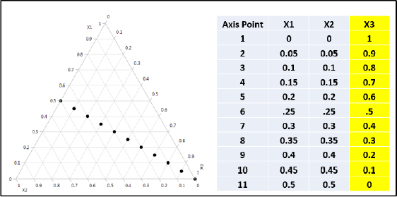
The summation constraint has the effect of modifying the geometry of the experimental region and reducing the dimensionality. This effect can be seen in Figure 1.1. Note that for two independent variables (non-formulations), the typical factorial designs are based on a two-dimensional square. With formulations, however, the second component must be one minus the first component. Hence, the available design space becomes a line instead of a square. Therefore, there is only one true dimension in the formulation design space, or one fewer than the dimensionality of the factorial space.

Figure 1.1 – Geometry of Formulation Experimental Regions

When experimenting with three independent (non-formulation) variables, the typical factorial designs are based on a three-dimensional cube. The three formulation components must sum to 1.0.  However, once the proportions of the first two components have been determined, the third must be 1.0 minus these. Therefore, the available design space becomes a two-dimensional triangle, or simplex. Chapter 3 discusses in detail the effect of the formulation constraint on the resulting experiment designs.

Displaying Formulation Compositions Using Trilinear Coordinates

The first effect of the formulation constraint is how the formulations are displayed graphically. This is particularly important as graphical display and analysis are critical to the successful design, analysis, and interpretation of formulation experiments and data. Trilinear coordinates are used to display formulation compositions. When all the components vary from 0 – 1, the region is referred to as a simplex. The region for three components is shown in Figures 1.2a, 1.2b, and 1.2c.

Figure 1.2a – Three-Component Simplex: x₁ Component Axis

Figure 1.2b – Three-Component Simplex: x₂ Component Axis

Figure 1.2c – Three-Component Simplex: x₃ Component Axis

The region is a triangle that has three vertices and three edges. The x₁ component axis runs vertically from the bottom (x₁=0) to the top (x₁=1) of the triangle (Figure 1.2a). The x₂ component axis varies from the right-hand side of Figure 1.2b (x₂=0) to the lower left of the figure (x₂=1).  The x₃ component axis varies from the left-hand side of Figure 1.2c (x₃=0) to the lower right of the figure (x₃=1).  Lines of constant x₁, x₂, and x₃ run parallel to the bottom, right, and left sides of the triangle, respectively. All coordinates of all the points in the figure sum to 1.0 (x₁+x₂+x₃=1).

The compositions of five formulations are shown in Figure 1.3.

Figure 1.3 – Trilinear Coordinates Examples

The point, or composition (0.7, 0.15, 0.15), is the intersection of the line x₁ = .7, which is 0.7 of the distance from the top and the bottom of the triangle; the line x₂ = 0.15, which is 0.15 of the distance from the right side to the left corner; and the line x₃ = .15, which is 0.15 of the distance from the left side to the lower right corner. In three-component mixtures, x₁ + x₂ + x₃  = 1. Hence, the third coordinate is one minus the sum of the other two. The resulting triangle has only two independent dimensions, and the intersection of any two lines defines a point. For example, the point (.4, .3, .3) is the intersection of the lines x₁ = .4 and x₂ = .3, or x₁ = .4 and x₃ = .3, or the intersection of x₂ = .3 and x₃ = .3. The use of trilinear coordinates to display formulations will be discussed further in Chapter 3 and used throughout the book.

In the case of more than three components (dimensions) the space is still referred to as a simplex. The constraint that the sum of the components (x’s) is a constant (in most cases 1) still holds.  As a result, the x’s cannot be varied independently of each other. In the case of q components, we can calculate the level of any component in the formulation, given the levels of the other components in the formulation. As a result, the regression model used to describe the data does not have an intercept term, and the quadratic (non-linear blending) model does not have squared terms. These models are discussed in detail in Chapter 4.

1.3 Formulation Case Studies

This section introduces four case studies to illustrate the problems addressed in formulation studies and how these problems are resolved. The methods to produce the designs, analyses, and results are discussed in the following chapters.

Food Product

Hare (1974) describes a three-component study whose objective was to study the blending behavior of three components on the performance of a vegetable oil as measured by the solid fat index (y). Ten formulations were prepared as summarized in Table 1.2 and displayed graphically in Figure 1.4.

Table 1.2 – Vegetable Oil Formulation Experimental Design Blends

Blend	Stearine	Vegetable Oil	Solids	Solid Fat Index
1	1	0	0	4.6
2	0	1	0	35.5
3	0	0	1	55.5
4	1/2	1/2	0	14.5
5	1/2	0	1/2	25.7
6	0	1/2	1/2	46.1
7	1/3	1/3	1/3	27.4
8	2/3	1/6	1/6	14.5
9	1/6	2/3	1/6	32.0
10	1/6	1/6	2/3	42.5

Figure 1.4 – Vegetable Oil Formulation Experimental Design

The three components were x₁=Stearine (vegetable oil solids of one type of oil), x₂=vegetable oil (a different oil type) and x₃=vegetable oil solids of yet a third type of oil. The objective of the experiment was to find compositions that would produce a solid fat index of 40.

Regression analysis was used to create the prediction equation that enables one to calculate the solid fat index for any composition of the three components studied:

E(y)= 4.61x₁ - 35.9x₂ + 56.0x₃ – 21.5x₁x₂ – 16.6x₁x₃

We note here that a cross-product term such as x₁x₂ describes the non-linear blending characteristics of components 1 and 2 (the response function is curved). It is not referred to as an interaction term as in models for process variables. Blending characteristics are discussed in detail in Chapter 4.

An effective way to understand the blending behavior of the components is to construct a response surface contour plot as shown in Figure 1.5.

Figure 1.5 – Vegetable Oil Contour Plot

Here we see that there are a number of compositions to choose from to produce a solid fat index of 40.

Formulation	Stearine (%)	Vegetable Oil (%)	Vegetable Oil Solids (%)	Predicted Solid Fat Index
1	10	45	45	40
2	20	15	65	40

In Table 1.2 we saw that Blend 10 (1/6, 1/6, 2/3) had a measured solid fat index of 42.5. We also saw that there are a number of possible tradeoffs between the components. The different components have different costs. The composition selected was the most cost effective formulation.

Pharmaceutical Tablet Formulation

Huisman et al. (1984) discuss the development of a pharmaceutical tablet containing up to three diluents: Alpha-Lactose Monohydrate, Potato Starch, and Anhydrous Alpha-Lactose. The lubricant Magnesium Stearate was held constant in the study.  The objective of the study was to find a formulation with tablet strength >80N (Newton) and disintegration time <60 seconds at minimum cost. The formulation design and response data are summarized in Table 1.3 and displayed in Figure 1.6.

Table 1.3 – Pharmaceutical Placebo Formulation Experiment Design

Blend	Alpha Lactose Monohydrate	Potato Starch	Anhydrous Alpha-Lactose	Tablet Strength	Disintegration Time
1	1	0	0	55.8	13
2	0	1	0	36.4	22
3	0	0	1	152.8	561
4	1/2	1/2	0	68.8	25
5	1/2	0	1/2	91	548
6	0	1/2	1/2	125	141
7	1/3	1/3	1/3	94.6	22
8	2/3	1/6	1/6	70.4	13
9	1/6	2/3	1/6	80	34
10	1/6	1/6	2/3	130	385

Figure 1.6 – Placebo Tablet Formulation Experiment Design

As we saw in Table 1.3, this study used the same formulation experiment design as the food product example discussed above. One major difference in this case is that there were two responses that needed to be considered: tablet strength and tablet disintegration time. It is typical that formulations will have several responses of interest.

Figure 1.7 shows the formulations that will meet the desired levels for strength and disintegration time--namely a region centered at a 1/3:1/3:1/3 (equal proportions) blend of Alpha-Lactose Monohydrate, Potato Starch, and Anhydrous Alpha-Lactose. When cost is considered, the blend chosen for the tablet would likely change depending on the cost of the components.

Figure 1.7 – Placebo Tablet Design Space

Lubricant Formulation

A group of chemical engineers were engaged in a lubricant blending study, whose objective was to determine how much of an additive to use to ensure that a formulation of three components would have the desired performance (Snee 1975). There were several uses for the formulation, each requiring a different amount of the additive. It was decided to conduct an experiment to generate data. The generated data would enable them to construct a prediction equation, and that equation would permit them to calculate the amount of additive needed to produce the desired performance for a given application.

Here are the four components and ranges studied:

•   x1 = Additive	0.07 - 0.18
•   x2 = Component A	0.00 – 0.30
•   x3 = Component B	0.37 – 0.70
•   x4 = Component C	0.00 – 0.15

These ranges were used to create an 18-blend extreme vertices design as shown in Table 1.4. The design included the viscosity (y) for each blend. Extreme vertices designs will be discussed in Chapters 7 and 8.

Table 1.4 – Lubricant Formulation Design

Blend	Additive	A	B	C	Viscosity
1	0.15	0	0.7	0.15	13.89
2	0.18	0.3	0.37	0.15	13.99
3	0.07	0.23	0.7	0	7.60
4	0.07	0.08	0.7	0.15	9.45
5	0.18	0.12	0.7	0	12.93
6	0.07	0.3	0.63	0	7.38
7	0.07	0.3	0.48	0.15	8.58
8	0.18	0	0.67	0.15	15.65
9	0.18	0.3	0.52	0	11.94
10	0.18	0	0.7	0.12	15.24
11	0.07	0.2275	0.6275	0.075	8.24
12	0.18	0.144	0.592	0.084	13.84
13	0.125	0.3	0.5	0.075	10.08
14	0.13	0.086	0.7	0.084	11.48
15	0.125	0.2375	0.6375	0	9.64
16	0.13	0.136	0.584	0.15	11.94
17	0.133	0.163	0.617	0.087	11.25
18	0.18	0.15	0.52	0.15	14.65

This data was used to generate the following 10-coefficient quadratic blending model:

E(y) = b₁x₁ + b₂x₂ + b₃x₃ + b₄x₄ + b₁₂x₁x₂ + b₁₃x₁x₃ + b₁₄x₁x₄ + b₂₃x₂x₃ + b₂₄x₂x₄ + b₃₄x₃x₄

Linear Blending	Non-Linear Blending	Non-Linear Blending
b1 = 126.9	b12 = -115.0	b23 = -5.80
b2 = 6.7	b13 = -99.0	b24 = -8.7
b3 = 7.0	b14 = -56.4	b34 = -6.7
b4 = 16.2

Given the levels of Components A, B, and C and the desired viscosity for a given application, the equation was used to calculate the amount of additive needed to create the desired formulation.

In Table 1.5 we see the results for the first eight applications of the model, which produced formulations for eight different customers.

Table 1.5 – Lubricant Application Blends

Batch	Additive	A	B	C	Y Obsd	Y Pred	Difference
1	0.0923	0.0741	0.6975	0.1361	10.35	10.32	0.03
2	0.1035	0.0846	0.6774	0.1345	10.8	10.75	0.05
3	0.1389	0.1244	0.6075	0.1292	12.2	12.22	-0.02
4	0.1793	0.1765	0.5211	0.1231	14.07	14.12	-0.05
5	0.1924	0.1936	0.4929	0.1211	14.72	14.8	-0.08
6	0.105	0.05	0.735	0.11	10.83	10.79	0.04
7	0.137	0.1	0.643	0.12	12.2	12.15	0.05
8	0.175	0.2	0.485	0.14	13.93	13.97	-0.04

The prediction standard deviation was 0.047, which was essentially equal to the viscosity measurement variation. The engineers were very pleased with the performance of the model and used it extensively in creating products for a variety of customers and applications.

Pharmaceutical Tablet Compactability

Martinello et al. (2006) describe a study that investigated a formulation involving the compound paracetamol, which was known to have poor flowability and compressibility properties. The study involved seven ingredients:

Component	Low Level	High Level
Microcel	0.50	0.88
KollydonVA64	0.10	0.25
Flowlac	0	0.25
KollydonCL30	0	0.10
PEG 400	0	0.10
Aerosil	0	0.03
MgSt	0.005	0.025

Nine responses were measured. Of particular interest were repose angle, compressibility, disintegration time, and friability (tendency of a pharmaceutical tablet to chip, crumble, or break). A 19-blend extreme vertices design shown in Table 1.6 was used to design the formulations to be tested.

Table 1.6 – Pharmaceutical Tablet Compactability Study Blends

Blend	Microcel	Kollydon VA64	Flowlac	Kollydon CL30	Peg  400	Aerosil	MgSt
1	0.58	0.165	0.125	0.05	0.05	0.015	0.015
2	0.615	0.25	0	0	0.1	0.03	0.005
3	0.5	0.25	0.245	0	0	0	0.005
4	0.5	0.25	0.025	0.1	0.1	0	0.025
5	0.595	0.25	0	0.1	0	0.03	0.025
6	0.5	0.1	0.245	0	0.1	0.03	0.025
7	0.875	0.1	0	0	0	0	0.025
8	0.58	0.165	0.125	0.05	0.05	0.015	0.015
9	0.5	0.1	0.245	0.1	0	0.03	0.025
10	0.525	0.1	0.25	0	0.1	0	0.025
11	0.865	0.1	0	0	0	0.03	0.005
12	0.595	0.25	0	0	0.1	0.03	0.025
13	0.58	0.165	0.125	0.05	0.05	0.015	0.015
14	0.5	0.25	0.245	0	0	0	0.005
15	0.695	0.1	0	0.1	0.1	0	0.005
16	0.58	0.165	0.125	0.05	0.05	0.015	0.015
17	0.695	0.1	0	0.1	0.1	0	0.005
18	0.515	0.1	0.25	0.1	0	0.03	0.005
19	0.58	0.165	0.125	0.05	0.05	0.015	0.015

A seven-term linear blending model was fit to the data and used to develop an optimal formulation. When tested, the formulation produced measured responses that were very close to those predicted by the linear blending model, as shown in Table 1.7. A linear blending model (only linear terms in the model) has a response function that is a straight line (two components) or a plane (> 2 components). Blending characteristics are discussed in detail in Chapter 4.

Table 1.7 – Pharmaceutical Tablet Compactability Optimal Formulation

Response	Predicted	Measured
Compressibility (%)	32.0	29.8
Water Content (%)	2.3	2.1
Repose Angle (deg)	21	18
Weight Variation (mg)	700	724
Hardness (kgf)	11.2	16.0
Friability (%)	1.03	0.91
Paracetamol Content (%)	99.7	97.4
Disintegration Time (min)	2.3	2.6
Dissolution (%)	91.9	92.0

The authors concluded “the optimal formulation showed good flowability, no lamination, and also met all official pharmaceutical specifications.” (Martinello et al, p. 95).

1.4 Summary and Looking Forward

In this chapter we have introduced a formulation as a product or entity produced by mixing or blending two or more components or ingredients. We have shown how experimenting with formulations is different from experimenting with process variables and other type of factors that can be varied independently of one another. Examples from different fields have been introduced, including four published applications that illustrate some of the problems formulators and formulation scientists encounter. In the next chapter we discuss the basics of experimentation that relate to formulations development.

1.5 References

Hare, L. B. (1974) “Mixture Designs Applied to Food Formulation.” Food Technology, 28 (3), 50-56, 62.

Snee, R. D. (1975) “Experimental Designs for Quadratic Models in Constrained Mixture Spaces.” Technometrics, 17 (2), 149-159.

Huisman, R., H. V. Van Kamp, J. W. Weyland, D. A. Doornbos, G. K. Bolhuis and C. F. Lerk. (1984) “Development and Optimization of Pharmaceutical Formulations using a Simplex Lattice Design.” Pharmaceutisch Weekblad, 6 (5), 185-194.

Kurotori, I. S. (1966) “Experiments with Mixtures of Components Having Lower Bounds.” Industrial Quality Control, 22 (11), May 1966, 592-596.

Martinello, T., T. M Kaneko, M. V. R. Velasco, M. E. S. Taqueda. And V. O. Consiglieri. (2006) “Optimization of Poorly Compactable Drug Tablets Manufactured by Direct Compression using the Mixture Experimental Design.” International Journal of Pharmaceutics, 322 (1-2), 87-95.

Wilkinson, N. B. (1966) Explosives in History: the Story of Black Powder. The Hagley Museum, Wilmington, DE.