
Chapter 13
Hydraulics
Contents
13.1 Introduction
13.2 Composition and Properties of Hydrocarbons
13.2.1 Hydrocarbon Composition
13.2.2 Equation of State
13.2.3 Hydrocarbon Properties
13.2.3.1 Density
13.2.3.2 Viscosity
13.3 Emulsion
13.3.1 General
13.3.2 Effect of Emulsion on Viscosity
13.3.3 Prevention of Emulsion
13.4 Phase Behavior
13.4.1 Black Oils
13.4.2 Volatile Oils
13.4.3 Condensate
13.4.4 Wet Gases
13.4.5 Dry Gases
13.4.6 Computer Models
13.5 Hydrocarbon Flow
13.5.1 General
13.5.2 Single-Phase Flow
13.5.2.1 Conservation Equations
13.5.2.2 Friction Factor Equation
13.5.2.3 Local Losses
13.5.3 Multiphase Flow
13.5.3.1 General
13.5.3.2 Horizontal Flow
13.5.3.3 Vertical Flow
13.5.4 Comparison of Two-Phase Flow Correlations
13.5.4.1 Description of Correlations
13.5.4.2 Analysis Method
13.6 Slugging and Liquid Handling
13.6.1 General
13.6.2 Hydrodynamic Slugging
13.6.3 Terrain Slugging
13.6.4 Start-Up and Blowdown Slugging
13.6.5 Rate Change Slugging
13.6.6 Pigging
13.6.7 Slugging Prediction
13.6.8 Parameters for Slug Characteristics![]() 386
386
13.6.9 Slug Detection and Control Systems
13.6.10 Equipment Design for Slug Flow
13.6.11 Slug Catcher Sizing
13.7 Slug Catcher Design
13.7.1 Slug Catcher Design Process
13.7.2 Slug Catcher Functions
13.7.2.1 Process Stabilization
13.7.2.2 Phase Separation
13.7.2.3 Storage
13.8 Pressure Surge
13.8.1 Fundamentals of Pressure Surge
13.8.2 Pressure Surge Analysis
13.9 Line Sizing
13.9.1 Hydraulic Calculations
13.9.2 Criteria
13.9.3 Maximum Operating Velocities
13.9.4 Minimum Operating Velocities
13.9.5 Wells
13.9.6 Gas Lift
13.1 Introduction
To ensure system deliverability of hydrocarbon products from one point in the flowline to another, the accurate prediction of the hydraulic behavior in the flowline is essential. From the reservoir to the end user, the hydrocarbon flow is impacted by the thermal behavior of the heat transfer and phase changes of the fluid in the system. The hydraulic analysis method used and its results are different for different fluid phases and flow patterns. To solve a hydrocarbon hydraulic problem with heat transfer and phase changes, adequate knowledge of fluid mechanics, thermodynamics, heat transfer, vapor/liquid equilibrium, and fluid physical properties for multicomponent hydrocarbon systems is needed. In this chapter, the composition and phase behavior of hydrocarbons are explained first. Then, the hydraulic analyses for single-phase flow and multiphase flow, which include pressure drop versus production flow rate and pipeline sizing, are discussed.
13.2 Composition and Properties of Hydrocarbons
13.2.1 Hydrocarbon Composition
The petroleum fluids from reservoirs normally are multiphase and multicomponent mixtures, primarily consisting of hydrocarbons, which can be classified into the following three groups:
In addition to hydrocarbons, water (H2O), nitrogen (N2), carbon dioxide (CO2), hydrogen sulfide (H2S), salts, and solids are often found in petroleum mixtures.
Table 13-1 lists some typical physical properties of the main components of petroleum. The boiling point of hydrocarbon components increases with an increase in the carbon number of the component formula. If the carbon number of a component is less than 5, the component is in the gas phase at atmospheric pressure. When the mixture contains larger molecules, it is a liquid at normal temperatures and pressures. A typical petroleum fluid contains thousands of different chemical compounds, and trying to separate it into different chemical homogeneous compounds is impractical. A composition of gas condensate is shown in Table 13-2. In the usual composition list of hydrocarbons, the last hydrocarbon is marked with a “+,” which indicates a pseudo-component, and lumps together all of the heavier components.
Table 13-1. Physical Properties of Main Petroleum Components [1]

Table 13-2. Typical Composition of a Gas Condensate [2]
| Component | Composition (mol %) | |
| Hydrogen sulfide | H2S | 0.05 |
| Carbon dioxide | CO2 | 6.50 |
| Nitrogen | N2 | 11.71 |
| Methane | C1 | 79.06 |
| Ethane | C2 | 1.62 |
| Propane | C3 | 0.35 |
| i-Butane | i-C4 | 0.08 |
| n-Butane | C4 | 0.10 |
| i-pentane | i-C5 | 0.04 |
| n-Pentane | C5 | 0.04 |
| Hexanes | C6 | 0.06 |
| Heptanes Plus | C7+ | 0.39 |
The characterization of a pseudo-component including its molecular weight, density, pseudo-critical properties, and other parameters should be calculated ahead of the flow assurance analysis (see Chapter 12). The characterization should be based on experimental data and analyses. As shown in Table 13-2, hydrocarbon isotropic compounds with the same formula and carbon atom numbers may have very different normal boiling points and other physical properties.
13.2.2 Equation of State
For oil and gas mixtures, the phase behavior and physical properties such as densities, viscosities, and enthalpies are uniquely determined by the state of the system. The equations of state (EOS) for petroleum mixtures are mathematical relations between volume, pressure, temperature, and composition, which are used for describing the system state and transitions between states. Most thermodynamic and transport properties in engineering analyses are derived from the EOS. Since 1873, when the first EOS for representation of real systems was developed by the van der Waals, hundreds of different EOSs have been proposed and they are distinguished by Leland [3] into four families:
The cubic equations of the van der Waals family are widely used in the oil and gas industry for engineering calculations because of their simplicity and relative accuracy for describing multiphase mixtures. The simple cubic equations of state, Soave-Redlich-Kwong (SRK) and Peng-Robinson (PR), are used in flow assurance software (e.g., PIPESIM). They require limited pure component data and are robust and efficient, and usually give broadly similar results.
The SRK Equation[4]
![]() (13-1)
(13-1)
where p is the pressure, T is the temperature, v is the molar volume, R is the gas constant, and a and b are the EOS constants, which are determined by the critical conditions for a pure component:
![]()
![]()
And m = 0.480 + 1.574 ω − 0.176 ω2, where ω is an acentric factor. For a mixture, a and b are found as follows:
![]()
![]()
where zi
and zj
are the mole fraction of components i and j, respectively, and ![]() , where kij
is a binary interaction coefficient, which is usually considered equal to zero for hydrocarbon/hydrocarbon interactions, and different from zero for interactions between a hydrocarbon and a nonhydrocarbon, and between unlike pairs of nonhydrocarbons.
, where kij
is a binary interaction coefficient, which is usually considered equal to zero for hydrocarbon/hydrocarbon interactions, and different from zero for interactions between a hydrocarbon and a nonhydrocarbon, and between unlike pairs of nonhydrocarbons.
PR Equation[5]
![]() (13-2)
(13-2)
The EOS constants are given by
![]()
![]()
and m = 0.3764 + 1.54226 ω − 0.26992 ω2, where ω is an acentric factor.
13.2.3 Hydrocarbon Properties
Oil and gas are very complex fluids composed of hydrocarbon compounds that exist in petroleum in a wide variety of combinations. Physical properties change with the component composition, pressure, and temperature. No two oils have the same physical properties. In considering hydrocarbon flow in pipes, the most important physical properties are density and viscosity.
13.2.3.1 Density
Dead oil is defined as oil without gas in solution. Its specific gravity γo is defined as the ratio of the oil density and the water density at the same temperature and pressure:
![]() (13-3)
(13-3)
API gravity, with a unit of degree (o) is defined as:
![]() (13-4)
(13-4)
where γo is the specific gravity of oil at 60°F, and the water density at 60°F is 62.37 lb/ft3.
The effect of gas dissolved in the oil should be accounted for in the calculation of the in situ oil (live oil) density. The oil density can be calculated as follows:
![]() (13-5)
(13-5)
where
Gas density ρg is defined as:
![]() (13-6)
(13-6)
where M is the molecular weight of the gas, R is the universal gas constant, p is the absolute pressure, T is the absolute temperature, and Z is the compressibility factor of gas. The gas specific gravity γg is defined as the ratio of the gas density and the air density at the same temperature and pressure:
![]() (13-7)
(13-7)
For liquids, the reference material is water, and for gases it is air.
13.2.3.2 Viscosity
Dynamic Viscosity
The dynamic viscosity of a fluid is a measure of the resistance to flow exerted by a fluid, and for a Newtonian fluid it is defined as:
![]() (13-8)
(13-8)
where τ is the shear stress, v is the velocity of the fluid in the shear stress direction, and dv/dn is the gradient of v in the direction perpendicular to flow direction.
Kinematic Viscosity
![]() (13-9)
(13-9)
The viscosity of Newtonian fluids is a function of temperature and pressure. If the viscosity of a fluid varies with the thermal or time history, the fluid is called non-Newtonian. Most of the hydrocarbon fluids are Newtonian fluid, but in some cases, the fluid in the flowline should be considered to be non-Newtonian. The viscosity of oil decreases with increasing temperature, while the viscosity of gas increases with increasing temperature. The general relations can be expressed as follows for liquids:
![]() (13-10)
(13-10)
and as follows for gases:
![]() (13-11)
(13-11)
where A, B, and C are constants determined from the experimental measurement. The viscosity typically increases with increased pressure for gas. The equation of viscosity can be expressed in terms of pressure as:
![]() (13-12)
(13-12)
The most commonly used unit to represent viscosity is the poise, which can be expressed as dyne · s/cm2 or g/cm · s. The centipoise or cP is equal to 0.01 poise. The SI unit of viscosity is Pa · s, which is equal to 0.1 poise. The viscosity of pure water at 20°C is 1.0 cP.
The viscosity of crude oil with dissolved gases is an important parameter for the calculation of pressure loss for hydrocarbon flow in pipeline [6]. Pressure drops of high viscous fluid along the pipeline segment may significantly impact deliverability of products. The oil viscosity should be determined in the laboratory for the required pressure and temperature ranges. Many empirical correlations are available in the literature that can be used to calculate the oil viscosity based on the system parameters such as temperature, pressure, and oil and gas gravities when no measured viscosity data are available.
To minimize pressure drop along the pipeline for viscous crude oils, it is beneficial to insulate the pipeline so it can retain a high temperature. The flow resistance is less because the oil viscosity is lower at higher temperatures. The selection of insulation is dependent on cost and operability issues. For most developed fields insulation may not be important. However, for heavy oil, high-pressure drops due to viscosity in the connecting pipeline between the subsea location and the receiving platform, insulation may have a key role to play.
13.3 Emulsion
13.3.1 General
A separate water phase in a pipeline system can result in hydrate formation or an oil/water emulsion under certain circumstances. Emulsions can have high viscosities, which may be an order of magnitude higher than the single-phase oil or water. The effect of emulsions on frictional loss may lead to a significantly larger error in pressure loss than calculated. In addition to affecting pipeline hydraulics, emulsions may present severe problems to downstream processing plants [7].
An emulsion is a heterogeneous liquid system consisting of two immiscible liquids with one of the liquids intimately dispersed in the form of droplets in the second liquid. In most emulsions of crude oil and water, the water is finely dispersed in the oil. The spherical form of the water globules is a result of interfacial tension, which compels them to present the smallest possible surface area to the oil. If the oil and water are violently agitated, small drops of water will be dispersed in the continuous oil phase and small drops of oil will be dispersed in the continuous water phase. If left undisturbed, the oil and water will quickly separate into layers of oil and water. If any emulsion is formed, it will exist between the oil above and the water below. In offshore engineering, most emulsions are the water-in-oil type.
The formation of an emulsion requires the following three conditions:
The agitation necessary to form an emulsion may result from any one or a combination of several sources:
• Flow through the tubing, wellhead, manifold, or flowlines;
• Pressure drop through chokes, valves, or other surface equipment.
The greater the amount of agitation, the smaller the droplets of water dispersed in the oil. Water droplets in water-in-oil emulsions are of widely varying sizes, ranging from less than 1 to about 1,000 μm. Emulsions that have smaller droplets of water are usually more stable and difficult to treat than those that have larger droplets. The most emulsified water in light crude oil, that is, oil above 20° API, is from 5 to 20 vol % water, while emulsified water in crude oil heavier than 20° API is from 10 to 35%. Generally, crude oils with low API gravity (high density) will form a more stable and higher percentage volume of emulsion than will oils of high API gravity (low density). Asphaltic-based oils have a tendency to emulsify more readily than paraffin-based oils.
The emulsifying agent determines whether an emulsion will be formed and the stability of that emulsion. If the crude oil and water contain no emulsifying agent, the oil and water may form a dispersion that will separate quickly because of rapid coalescence of the dispersed droplets. Emulsifying agents are surface-active compounds that attach to the water-drop surface. Some emulsifiers are thought to be asphaltic, sand, silt, shale particles, crystallized paraffin, iron, zinc, aluminum sulfate, calcium carbonate, iron sulfide, and similar materials. These substances usually originate in the oil formation but can be formed as the result of an ineffective corrosion-inhibition program.
13.3.2 Effect of Emulsion on Viscosity
Emulsions are always more viscous than the clean oil contained in the emulsion.
Figure 13-1 shows the tendency of viscosity with the increase of water cut in different emulsion conditions. This relationship was developed by Woelflin [8] and is widely used in petroleum engineering. However, at higher water cuts (greater than about 40%), it tends to be excessively pessimistic and may lead to higher pressure loss expectations than are actually likely to occur. Guth and Simha [9] presented a correlation of emulsion viscosity:
![]() (13-13)
(13-13)

Figure 13-1 Woelflin Viscosity Data
where μe is the viscosity of emulation (in cP or mPa·s), μo is the viscosity of clean oil (cP or mPa·s), Cw is the volume fraction of the water phase, it is a ration of water volumetric flow rate compared to the volumetric flow rate of total liquids, including oil, water and other liquids.
This correlation is similar to that of Woelflin in that it predicts the emulsion viscosity to be some multiple of the oil viscosity. The factor is determined solely as a function of the water cut. Up to a water cut of about 40%, the two methods will give almost identical results. Above that, the effective viscosity rises much more slowly with the Guth and Simha [9] correlation, and computed pressure losses will thus be lower at higher water cuts.
Laboratory tests can provide useful information about emulsions, but the form of the emulsion obtained in practice is dependent on the shear history, temperature, and composition of the fluids. Limited comparison of calculated emulsion viscosity with experimental data suggests that the Woelflin correlation overestimates the viscosity at higher water fractions. The following equation, from by Smith and Arnold [10] can be used if no other data are available:
![]() (13-14)
(13-14)
13.3.3 Prevention of Emulsion
If all water can be excluded from the oil and/or if all agitation of hydraulic fluid can be prevented, no emulsion will form. Exclusion of water in some wells is difficult or impossible, and the prevention of agitation is almost impossible. Therefore, production of emulsion from many wells must be expected. In some instances, however, emulsification is increased by poor operating practices.
Operating practices that include the production of excess water as a result of poor cementing or reservoir management can increase emulsion-treating problems. In addition, a process design that subjects the oil/water mixture to excess turbulence can result in greater treatment problems. Unnecessary turbulence can be caused by overpumping and poor maintenance of plunger and valves in rod-pumped wells, use of more gas-lift gas than is needed, and pumping the fluid when gravity flow could be used instead. Some operators use progressive cavity pumps as opposed to reciprocating, gear, or centrifugal pumps to minimize turbulence. Others have found that some centrifugal pumps can actually cause coalescence if they are installed in the process without a downstream throttling valve. Wherever possible, pressure drop through chokes and control valves should be minimized before oil/water separation.
13.4 Phase Behavior
A multicomponent mixture exhibits an envelope for liquid/vapor phase change in the pressure/temperature diagram, which contains a bubble-point line and a dew-point line, compared with only a phase change line for a pure component. Figure 13-2 shows the various reservoir types of oil and gas systems based on the phase behavior of hydrocarbons in the reservoir, in which the following five types of reservoirs are distinguished:

Figure 13-2 Typical Phase Diagram of Hydrocarbons
The amount of heavier molecules in the hydrocarbon mixtures varies from large to small in the black oils to the dry gases, respectively. The various pressures and temperatures of hydrocarbons along a production flowline from the reservoir to separator are presented in curve A–A2 of Figure 13-2. Mass transfer occurs continuously between the gas and the liquid phases within the two-phase envelope.
13.4.1 Black Oils
Black oil is liquid oil and consists of a wide variety of chemical species including large, heavy, and nonvolatile molecules. Typical black oil reservoirs have temperatures below the critical temperature of a hydrocarbon mixture. Point C in Figure 13-2 represents unsaturated black oil; some gases are dissolved in the liquid hydrocarbon mixture. Point C1 in the same figure shows saturated back oil, which means that the oil contains as much dissolved gas as it can take and that a reduction of system pressure will release gas to form the gas phase. In transport pipelines, black oils are transported in the liquid phase throughout the transport process, whereas in production flowlines, produced hydrocarbon mixtures are usually in thermodynamical equilibrium with gas.
13.4.2 Volatile Oils
Volatile oils contain fewer heavy molecules than black oil, but more ethane through hexane. Reservoir conditions are very close to the critical temperature and pressure. A small reduction in pressure can cause the release of a large amount of gas.
13.4.3 Condensate
Retrograde gas is the name of a fluid that is gas at reservoir pressure and temperature. However, as pressure and temperature decrease, large quantities of liquids are formed due to retrograde condensation. Retrograde gases are also called retrograde gas condensates, gas condensates, or condensates. The temperature of condensates is normally between the critical temperature and the cricondentherm as shown in Figure 13-2. From reservoir to riser top, as shown in points B to B2 in the figure, the fluid changes from single gas and partial transfer to condensate liquid and evaporate again as gas, causing a significant pressure drop.
For a pure substance a decrease in pressure causes a change of phase from liquid to gas at the vapor–pressure line; likewise, in the case of a multicomponent system, a decrease in pressure causes a change of phase from liquid to gas at temperatures below the critical temperature. However, consider the isothermal decrease in pressure illustrated by a line B–B1–B2 in Figure 13-2. As pressure is decreased from point B, the dew-point line is crossed and liquid begins to form. At the position indicated by point B1, the system is 5% liquid. A decrease in pressure has caused a change from gas to liquid. Table 13-3 lists the composition of a typical condensate gas. Curve A–A2 illustrates the variations of pressure and temperature along the flowline from reservoir to the separator on a platform.
13.4.4 Wet Gases
A wet gas exists in a pure gas phase in the reservoir, but becomes a liquid/gas two-phase mixture in a flowline from the well tube to the separator at the topside platform. During the pressure drop in the flowline, liquid condensate appears in the wet gas.
13.4.5 Dry Gases
Dry gas is primarily methane. The hydrocarbon mixture is solely gas under all conditions of pressure and temperature encountered during the production phases from reservoir conditions involving transport and process conditions. In particular, no hydrocarbon-based liquids are formed from the gas although liquid water can condense. Dry gas reservoirs have temperatures above the cricondentherm. Tables 13-3 and 13-4 list the hydrocarbon composition and properties, respectively, of typical reservoirs.
Table 13-3. Hydrocarbon Composition of Typical Reservoirs [11]

Table 13-4. Hydrocarbon Properties of Typical Reservoirs [11]

13.4.6 Computer Models
Accurate prediction of physical and thermodynamic properties is a prerequisite to successful pipeline design. Pressure loss, liquid hold up, heat loss, hydrate formation, and wax deposition all require knowledge of the fluid states.
In flow assurance analyses, the following two approaches have been used to simulate hydrocarbon fluids:
• “Black-oil” model: Defines the oil as a liquid phase that contains dissolved gas, such as hydrocarbons produced from the oil reservoir. The “black oil” accounts for the gas that dissolves (condenses) from oil solution with a parameter of Rs that can be measured from the laboratory. This model predicts fluid properties from the specific gravity of the gas, the oil gravity, and the volume of gas produced per volume of liquid. Empirical correlations evaluate the phase split and physical property correlations determine the properties of the separate phases.
• Composition model: For a given mole fraction of a fluid mixture of volatile oils and condensate fluids, a vapor/liquid equilibrium calculation determines the amount of the feed that exists in the vapor and liquid phases and the composition of each phase. It is possible to determine the quality or mass fraction of gas in the mixtures. Once the composition of each phase is known, it is also possible to calculate the interfacial tension, densities, enthalpies, and viscosities of each phase.
The accuracy of the compositional model is dependent on the accuracy of the compositional data. If good compositional data are available, selection of an appropriate EOS is likely to yield more accurate phase behavior data than the corresponding black-oil model. This is particularly so if the hydrocarbon liquid is a light condensate. In this situation complex phase effects such as retrograde condensation are unlikely to be adequately handled by the black-oil methods. Of prime importance to hydraulic studies is the viscosity of the fluid phases. Both black-oil and compositional techniques can be inaccurate. Depending on the correlation used, very different calculated pressure losses could result. With the uncertainty associated with viscosity prediction, it is prudent to utilize laboratory-measured values.
The gas/oil ratio (GOR) can be defined as the ratio of the measured volumetric flow rates of the gas and oil phases at meter conditions (multiphase meter) or the volume ratio of gas and oil at the standard condition (1 atm, 60°F) in units of scf/STB. When water is also present, the water cut is generally defined as the volume ratio of the water and total liquid at standard conditions. If the water contains salts, the salt concentrations may be contained in the water phase at the standard condition.
13.5 Hydrocarbon Flow
13.5.1 General
The complex mixture of hydrocarbon compounds or components can exist as a single-phase liquid, a single-phase gas, or as a multiphase mixture, depending on its pressure, temperature, and the composition of the mixture. The fluid flow in pipelines is divided into three categories based on the fluid phase condition:
• Single-phase condition: black oil or dry gas transport pipeline, export pipeline, gas or water injection pipeline, and chemical inhibitors service pipelines such as methanol and glycol lines;
• Two-phase condition: oil + released gas flowline, gas + produced oil (condensate) flowline
• Three-phase condition: water + oil + gas (typical production flowline).
The pipelines after oil/gas separation equipment, such as transport pipelines and export pipelines, generally flow single-phase hydrocarbon fluid while in most cases, the production flowlines from reservoirs have two- or three-phase fluids, simultaneously, and the fluid flow is then called multiphase flow.
In a hydrocarbon flow, the water should be considered as a sole liquid phase or in combination with oils or condensates, since these liquids basically are insoluble in each other. If the water amount is small enough that it has little effect on flow performance, it may be acceptable to assume a single liquid phase. At a low-velocity range, there is considerable slip between the oil and water phases. As a result, the water tends to accumulate in low spots in the system. This leads to high local accumulations of water and, therefore, a potential for water slugs in the flowline. It may also cause serious corrosion problems.
Two-phase (gas/liquid) models are used for black-oil systems even when water is present. The water and hydrocarbon liquid are treated as a combined liquid with average properties. For gas condensate systems with water, three-phase (gas/liquid/aqueous) models are used.
The hydraulic theory underlying single-phase flow is well understood and analytical models may be used with confidence. Multiphase flow is significantly more complex than single-phase flow. However, the technology to predict multiphase-flow behavior has improved dramatically in the past decades. It is now possible to select pipeline size, predict pressure drop, and calculate flow rate in the flowline with an acceptable engineering accuracy.
13.5.2 Single-Phase Flow
The basis for calculation of changes in pressure and temperature with pipeline distance is the conservation of mass, momentum, and energy of the fluid flow. In this section, the steady-state, pressure-gradient equation for single-phase flow in pipelines is developed. The procedures to determine values of wall shear stress are reviewed and example problems are solved to demonstrate the applicability of the pressure-gradient equation for both compressible and incompressible fluid. A review is presented of Newtonian and non-Newtonian fluid flow behavior in circular pipes. The enthalpy-gradient equation is also developed and solved to obtain approximate equations that predict temperature changes during steady-state fluid flow.
13.5.2.1 Conservation Equations
Mass Conservation
Mass conservation of flow means that the mass in, min , minus the mass out, mout , of a control volume must equal the mass accumulation in the control volume. For the control volume of a one-dimensional pipe segment, the mass conservation equation can be written as:
![]() (13-15)
(13-15)
where ρ is the fluid density, v is the fluid velocity, t is the time, and L is the length of the pipe segment. For a steady flow, no mass accumulation occurs, and Equation (13-15) becomes:
![]() (13-16)
(13-16)
Momentum Conservation
Based on Newton’s second law applied to fluid flow in a pipe segment, the rate of momentum change in the control volume is equal to the sum of all forces on the fluid. The linear momentum conservation equation for the pipe segment can be expressed as:
![]() (13-17)
(13-17)
The terms on the right-hand side of Equation (13-17) are the forces on the control volume. The term ∂p/∂L represents the pressure gradient, τπd/A represents the surface forces, and ρg sin θ represents the body forces. Combining Equations (13-16) and (13-17), the pressure gradient equation is obtained for a steady-state flow:
![]() (13-18)
(13-18)
By integrating both sides of the above equation from section 1 to section 2 of the pipe segment shown in Figure 13-3, and adding the mechanical energy by hydraulic machinery such as a pump, an energy conservation equation, the Bernoulli equation, for a steady one-dimensional flow is obtained as:
![]() (13-19)
(13-19)

Figure 13-3 Relationship between Energy/Hydraulic Grade Lines and Individual Heads [12]
where, p/γ is pressure head; V2/2g is velocity head, z is elevation head, ∑hf is the sum of the friction head loss between section 1 and 2 caused by frictional force, ∑hl is the sum of the local head loss, and hm is mechanical energy per unit weight added by hydraulic machinery. The pipe friction head loss is the head loss due to fluid shear at the pipe wall. The local head losses are caused by local disruptions of the fluid stream, such as valves, pipe bends, and other fittings.
The energy grade line (EGL) is a plot of the sum of the three terms in the left-hand side of Equation (13-19), and is expressed as:
![]() (13-20)
(13-20)
The hydraulic grade line (HGL) is the sum of only the pressure and elevation head, and can be expressed as:
![]() (13-21)
(13-21)
Figure 13-3 shows the relation of the individual head terms to the EGL and HGL lines. The head losses represent the variation of EGL or HGL between section 1 and 2. In general, in a preliminary design, the local losses may be ignored, but they must be considered at the detailed design stage.
As shown in Equation (13-19), the total pressure drop in a particular pipe segment is the sum of the friction head losses of the pipe segment, valves, and fittings, the local head losses due to valves and fittings, the static pressure drop due to elevation change, and the pressure variation due to the acceleration change.
13.5.2.2 Friction Factor Equation
The Darcy-Weisbach equation is one of the most general friction head loss equations for a pipe segment. It is expressed as:
![]() (13-22)
(13-22)
![]() (13-23)
(13-23)
where f is the friction factor, Re = VDρ/μ is the Reynolds number, and ε/D is the equivalent sand-grain roughness (relative roughness) of the pipe, which is decided by the pipeline material. Figure 13-4 shows the graphical representation of the friction factor at different flow regions, which is also called as Moody diagram.

Figure 13-4 Moody Diagram [13]
Table 13-5 lists common values of absolute roughness for several materials. For steel pipe, the absolute roughness is 0.0018 in. unless alternative specifications are specified. The absolute roughness of 0.0018 in. is for aged pipe, but that is accepted in design practice because it is conservative. Flexible pipe is rougher than steel pipe and, therefore, requires a larger diameter for the same maximum rate. For a flexible pipe, the roughness is given by ε = ID/250.0 unless an alternative specification is given. The roughness may increase with use at a rate determined by the material and nature of the fluid. As a general guide, factors of safety of 20% to 30% on the friction factor will accommodate the change in roughness conditions for steel pipe with average service of 5 to 10 years.
Table 13-5. Pipeline Material Roughness [14]
| Material | ε, Equivalent Sand-Grain Roughness (in.) |
| Concrete | 0.012–0.12 |
| Case iron | 0.010 |
| Commercial or welded steel | 0.0018 |
| PVC, glass | 0.00006 |
As shown in Figure 13-4, the function f (Re, ε/D) is very complex. A laminar region and a turbulent region are defined in the Moody diagram based on the flow characteristics.
Laminar Flow
In laminar flow (Re < 2100), the friction factor function is a straight line and is not influenced by the relative roughness:
![]() (13-24)
(13-24)
The friction head loss is shown to be proportional to the average velocity in the laminar flow. Increasing pipe relative roughness will cause an earlier transition to turbulent flow. When the Reynolds number is in the range from 2000 to 4000, the flow is in a critical region where it can be either laminar or turbulent depending on several factors. These factors include changes in section or flow direction. The friction factor in the critical region is indeterminate, which is in a range between friction factors for laminar flow and for turbulent flow.
Turbulent Flow
When the Reynolds number is larger than 4000, the flow inside the pipe is turbulent flow; the fiction factor depends not only on the Reynolds number but also on the relative roughness, ε/D, and other factors. In the complete turbulence region, the region above a dashed line in the upper right part of a Moody diagram, friction factor f is a function only of roughness ε/D. For a pipe in the transition zone, the friction factor decreases rapidly with increasing Reynolds number and decreasing pipe relative roughness. The lowest line in Figure 13-4 is the line representing the friction factor for the smoothest pipe, where the roughness ε/D is so small that it has no effect.
Although single-phase flow in pipes has been studied extensively, it still involves an empirically determined friction factor for turbulent flow calculations. The dependence of this friction factor on pipe roughness, which must usually be estimated, makes the calculated pressure gradients subject to considerable error and summarizes the correlations of Darcy-Weisbach friction factor for different flow ranges. The correlations for smooth pipe and complete turbulence regions are simplified from the one for a transitional region. For smooth pipe, the relative roughness term is ignored, whereas for the complete turbulence region, the Reynolds term is ignored.
Table 13-6 summarizes some Darcy-Weisbach friction factor correlations for both laminar flow and turbulent flow.
Table 13-6. Darcy-Weisbach Friction Factor Correlations [12]
| Flow Region | Friction Factor, f | Reynolds Range |
| Laminar | Re < 2100 | |
| Smooth pipe | Re > 4000 and ε/D →0 | |
| Transitional, Colebrook-White correlation | Re > 4000 and transitional region | |
| Complete turbulence | Re > 4000 and complete turbulence |
13.5.2.3 Local Losses
In addition to pressure head losses due to pipe surface friction, the local losses are the pressure head loss occurring at flow appurtenances, such as valves, bends, and other fittings, when the fluid flows through the appurtenances. The local head losses in fittings may include:
• Direction change of flow path;
• Sudden or gradual changes in the cross section and shape of the flow path.
The local losses are considered minor losses. These descriptions are misleading for the process piping system where fitting losses are often much greater than the losses in straight piping sections. It is difficult to quantify theoretically the magnitudes of the local losses, so the representation of these losses is determined mainly by using experimental data. Local losses are usually expressed in a form similar to that for the friction loss. Instead of f L/D in friction head loss, the loss coefficient K is defined for various fittings. The head loss due to fitting is given by the following equation:
![]() (13-25)
(13-25)
where V is the downstream mean velocity normally. Two methods are used to determine the value of K for different fittings, such as a valve, elbow, etc. One method is to choose a K value directly from a table that is invariant with respect to size and Reynolds number.
Table 13-7 gives K values for several types of fittings. In this method the data scatter can be large, and some inaccuracy is to be expected. The other approach is to specify K for a given fitting in terms of the value of the complete turbulence friction factor fT for the nominal pipe size. This method implicitly accounts for the pipe size. The Crane Company’s Technical Paper 410 [15] detailed the calculation methods for the K value for different fittings, and they are commonly accepted by the piping industry.
Table 13-7. Loss Coefficients for Fittings [15]
| Fitting | K |
| Globe valve, fully open | 10.0 |
| Angle valve, fully open | 5.0 |
| Butterfly valve, fully open | 0.4 |
| Gate valve, full open | 0.2 |
| 3/4 open | 1.0 |
| 1/2 open | 5.6 |
| 1/4 open | 17.0 |
| Check valve, swing type, fully open | 2.3 |
| Check valve, lift type, fully open | 12.0 |
| Check valve, ball type, fully open | 70.0 |
| Elbow, 45° | 0.4 |
| Long radius elbow, 90° | 0.6 |
Manufacturers of valves, especially control valves, express valve capacity in terms of a flow coefficient Cv , which gives the flow rate through the valve in gal/min of water at 60°F under a pressure drop of 1.0 psi. It is related to K by:
![]() (13-26)
(13-26)
where d is the diameter of the valve connections in inches.
13.5.3 Multiphase Flow
13.5.3.1 General
Multiphase transport is currently receiving much attention throughout the oil and gas industry, because the combined transport of hydrocarbon liquids and gases, immiscible water, and sand can offer significant economic savings over the conventional, local, platform-based separation facilities. However, the possibility of hydrate formation, the increasing water content of the produced fluids, erosion, heat loss, and other considerations create many challenges to this hydraulic design procedure.
Much research has been carried out on two-phase flow beginning in the 1950s. The behavior of two-phase flow is much more complex than that of single-phase flow. Two-phase flow is a process involving the interaction of many variables. The gas and liquid phases normally do not travel at the same velocity in the pipeline because of the differences in density and viscosities. For an upward flow, the gas phase, which is less dense and less viscous, tends to flow at a higher velocity than the liquid phase. For a downward flow, the liquid often flows faster than the gas because of density differences. Although analytical solutions of single-phase flow are available and the accuracy of prediction is acceptable in industry, multiphase flows, even when restricted to a simple pipeline geometry, are in general quite complex.
Calculations of pressure gradients in two-phase flows require values of flow conditions, such as velocity, and fluid properties, such as density, viscosity, and surface tension. One of the most important factors to consider when determining the flow characteristics of two-phase flows is flow pattern. The flow pattern description is not merely an identification of laminar or turbulent flow for a single flow; the relative quantities of the phases and the topology of the interfaces must also be described. The different flow patterns are formed because of relative magnitudes of the forces that act on the fluids, such as buoyancy, turbulence, inertia, and surface tension forces, which vary with flow rates, pipe diameter, inclination angle, and the fluid properties of the phases. Another important factor is liquid holdup, which is defined as the ratio of the volume of a pipe segment occupied by liquid to the volume of the pipe segment. Liquid holdup is a fraction, which varies from zero for pure gas flow to one for pure liquid flow.
For a two-phase flow, most analyses and simulations solve mass, momentum, and energy balance equations based on one-dimensional behavior for each phase. Such equations, for the most part, are used as a framework in which to interpret experimental data. Reliable prediction of multiphase flow behavior generally requires use of data or experimental correlations. Two-fluid modeling is a developing technique made possible by improved computational methods. In fluid modeling, the full three-dimensional partial differential equations of motion are written for each phase, treating each as a continuum and occupying a volume fraction that is a continuous function of position,
13.5.3.2 Horizontal Flow
In horizontal pipe, flow patterns for fully developed flow have been reported in numerous studies. Transitions between flow patterns are recorded with visual technologies. In some cases, statistical analysis of pressure fluctuations has been used to distinguish flow patterns. Figure 13-5 shows a typical flow pattern map, which gives an approximate prediction of the flow patterns. Commonly used flow pattern maps such as those of Mandhane and Baker are based on observed regimes in horizontal, small-diameter, air/water systems. Scaling to the conditions encountered in the oil and gas industries is uncertain.

Figure 13-5 Flow Pattern Regions for Two-phase Flow through Horizontal Pipe [16]
Figure 13-6 shows seven flow patterns for horizontal gas/liquid two-phase flow:
• Bubble flow: Gas is dispersed as bubbles that move at a velocity similar to that of liquid and tend to concentrate near the top of the pipe at lower liquid velocities.
• Plug flow: Alternate plugs of gas and liquid move along the upper part of the pipe.
• Stratified flow: Liquid flows along the bottom of the pipe and the gas flows over a smooth liquid/gas interface.
• Wavy flow: Occurs at greater gas velocities and has waves moving in the flow direction. When wave crests are sufficiently high to bridge the pipe, they form frothy slugs that move at much greater than the average liquid velocity.
• Slug flow: May cause severe and/or dangerous vibrations in equipment because of the impact of the high-velocity slugs against fittings.
• Annular flow: Liquid flows as a thin film along the pipe wall and gas flows in the core. Some liquid is entrained as droplets in the gas core.
• Spray: At very high gas velocities, nearly all the liquid is entrained as small droplets. This pattern is also called dispersed or mist flow.

Figure 13-6 Two-Phase Flow Patterns in Horizontal Pipeline [17]
13.5.3.3 Vertical Flow
Two-phase flow in vertical pipe may be categorized into four different flow patterns, as shown in Figure 13-7 and listed here:
• Bubble flow: The liquid is continuous, with the gas phase existing as randomly distributed bubbles. The gas phase in bubble flow is small and contributes little to the pressure gradient except by its effect on the density.
• Slug flow: Both the gas and liquid phases significantly contribute to the pressure gradient. The gas phase in slug flow exists as large bubbles and is separated by slugs of liquid. The velocity of the gas bubbles is greater than that of the liquid slugs, thereby resulting in a liquid holdup that not only affects well and riser friction losses but also flowing density.
• Churn flow: The liquid slugs between the gas bubbles essentially disappear and at some point the liquid phase becomes discontinuous and the gas phase becomes continuous. The pressure losses are more the result of the gas phase than the liquid phase.
• Annular flow: This type of flow is characterized by a continuous gas phase with liquid occurring as entrained droplets in the gas stream and as a liquid film wetting the pipe wall.

Figure 13-7 Two-Phase Flow Patterns in Vertical Pipe [18]
13.5.4 Comparison of Two-Phase Flow Correlations
Many two-phase flow correlations have been developed in past several decades, most of which are based on water/air systems, and every correlation has its limit because of the data used. Most software used in flow assurance has several options for models or correlations for two-phase flow. Baker Jardine [19] conducted a major data matching study to identify the most suitable two-phase flow correlations for oil wells, condensate wells, oil pipelines, and gas/condensate pipelines, and the results of the analysis are summarized in following sections.
13.5.4.1 Description of Correlations
Duns and Ros (D-R)
The Duns and Ros correlation [20] was developed for vertical two-phase flow in wells based on extensive experimental research on oil and air mixtures. Separate correlations were developed for bubble, plug, and froth flows, slug flows, and mist flow regimes. These regions have low, intermediate, and high gas throughputs, respectively.
Orkiszewski (OR)
The Orkiszewski correlation [21] was developed for the prediction of two-phase pressure drops in vertical pipe. The bubble, slug, annular-slug transition, and annular mist flow regimes were considered. The method can accurately predict within 10% the two-phase pressure drops in flowing and gas-lift production wells over a wide range of well conditions based on 148 measured pressure drops.
Hagedorn and Brown (H-B)
The Hagedorn and Brown correlation [22] was developed based on an experimental study of pressure gradients in small-diameter vertical conduits. A 1500-ft experimental well was used to study flow through 1-in., 1.25-in., and 1.5-in. nominal size tubing for widely varying liquid flow rates, gas/liquid ratios, and liquid viscosities.
Beggs and Brill Original (B-BO)
The Beggs and Brill correlation [17] was developed following a study of two-phase flow in horizontal and inclined pipe. The correlation is based on a flow regime map. The model inclines flow both upward and downward at angles of up to ±90°.
Beggs and Brill Revised (B-BR)
The enhancements to the original method [17] are as follows: (1) An extra flow regime is considered that assumes a no-slip holdup, and (2) the friction factor was changed from the standard smooth pipe model to one that utilizes a single-phase friction factor based on the average fluid velocity.
Mukherjee and Brill (M-B)
The Mukherjee and Brill correlation [23] was developed following a study of pressure drop in two-phase inclined flow. Results agreed well with the experimental data, and correlations were further verified with Prudhoe Bay and North Sea data.
Govier, Aziz, and Fogarasi (G-A)
The Govier, Aziz, and Fogarasi correlation [24] was developed following a study of pressure drop in wells producing gas and condensate. Actual field pressure drop versus flow rate data from 102 wells with gas/liquid ratios ranging from 3,900 to 1,170,000 scf/bbl were analyzed in detail.
No-Slip (NS)
The no-slip correlation assumes homogeneous flow with no slippage between the phases. Fluid properties are taken as the average of the gas and liquid phases, and friction factors are calculated using the single-phase Moody correlation.
OLGAS-89 and OLGAS 92 (O-89, O-92)
OLGAS [25] is based on data from the SINTEF two-phase flow laboratory. The test facilities were designed to operate at conditions similar to field conditions. The test loop was 800 m long and had an 8-in. diameter. Operating pressures were between 20 barg and 90 barg. Gas superficial velocities of up to 13 m/s and liquid superficial velocities of up to 4 m/s were obtained. Pipeline inclination angles between ±1° were studied in addition to flow up or down a hill section ahead of a 50-m-high vertical riser. More than 10,000 experiments were run on the test loop. OLGAS considers four flow regimes: stratified, annular, slug, and dispersed bubble flow.
Ansari (AN)
The Ansari model [26] was developed as part of the Tulsa University Fluid Flow Project (TUFFP) research program. A comprehensive model was formulated to predict flow patterns and the flow characteristics of the predicted flow patterns for upward two-phase flow. The model was evaluated by using the TUFFP well data bank that is composed of 1775 well cases, with 371 of them from Prudhoe Bay data.
BJA for Condensates (BJ)
Baker Jardine & Associates have developed a correlation [27] for two-phase flow in gas/condensate pipelines with a no-slip liquid volume fraction of lower than 0.1. The pressure loss calculation procedure is similar in approach to that proposed by Oliemans (see below), but accounts for the increased interfacial shear resulting from the liquid surface roughness.
AGA and Flanigan (AGA)
The AGA and Flanigan correlation [28] was developed for horizontal and inclined two-phase flow of gas/condensate systems. The Taitel Dukler flow regime map is used, which considers five flow regimes: stratified smooth, stratified wavy, intermittent, annular dispersed liquid, and dispersed bubble [29].
Oliemans (OL)
The Oliemans correlation [30] was developed following the study of large-diameter condensate pipelines. The model was based on a limited amount of data from a 30-in., 100-km pipeline operating at pressures of 100 barg or higher.
Gray (GR)
This correlation was developed by H. E. Gray [31] of Shell Oil Company for vertical flow in gas and condensate systems that are predominantly gas phase. Flow is treated as single phase, and water or condensate is assumed to adhere to the pipe wall. It is considered applicable to vertical flow cases where the velocity is below 50 ft/s, the tube size is below 3½ in., the condensate ratio is below 50 bbl/mmscf, and the water ratio is below 5 bbl/mmscf.
Xiao (XI)
The Xiao comprehensive mechanistic model [32] was developed as part of the TUFPP research program. It was developed for gas/liquid two-phase flow in horizontal and near horizontal pipelines. The data bank included large-diameter field data culled from the AGA multiphase pipeline data bank and laboratory data published in the literature. Data included both black oil and compositional fluid systems. A new correlation was proposed that predicts the internal friction factor under stratified flow.
13.5.4.2 Analysis Method
The predictions of pressure drop and flow rate for each of the correlations built in PIPESIM were compared with available experimental data from well/pipeline tests, reservoir fluid analysis, and drilling surveys/pipeline measurements collected by Baker Jardine. The percentage error for data points is calculated by:
![]()
Table 13-8 lists the evaluation method with scores for each correlation. The overall scores for pressure drop and flow rate predictions are averaged for each correlation. The score is calculated with the sum of score for each database divided by 3 × the total database number. The evaluation results for each correlation with a database of vertical oil wells, highly deviated oil wells, gas-condensate wells, oil pipelines, and gas-condensate pipelines are demonstrated in Figure 13-8.
Table 13-8. Evaluation of Correlations with Score [33]
| Error Range (%) | Evaluation | Score |
| – 5.0 to + 5.0 | Very good | 3.0 |
| –10.0 to + 10.0 | Good | 2.0 |
| –20.0 to + 20.0 | Moderate | 0 |
| Outside above range | Poor | –3.0 |

Figure 13-8 Evaluation of the Two-Phase Flow Correlations Used in PIPESIM
The Moody correlation is recommended for single-phase flow in vertical oil flow, horizontal oil flow, vertical gas flow, and horizontal gas flow.
13.6 Slugging and Liquid Handling
13.6.1 General
The occurrence of slug flow in a transportation pipeline can cause many problems in design and operation processes, which include kinetic force on fittings and vessels, pressure cycling, control instability, and inadequate phase separation. Slugging greatly affects the design of receiving facilities. In gas-condensate systems, larger lines result in more liquid being retained in the pipeline at low rates. When the flow rate is increased, much of the liquid can be swept out, potentially overwhelming the liquid handling capability of the receiving facilities. The facilities can be flooded and damaged if the slugs are larger than the slug catcher capacity. Therefore, quantifying the slug size, frequency, and velocity is necessary prior to equipment design.
The pressure at the bottom of the riser can vary if the holdup in the riser is not about the same as that in the line feeding it. If the riser holdup is too large and the gas velocity is too small to provide continuous liquid lift, too much of the liquid reverses and flows downward. Liquid accumulates at the base, causing an unstable pressure situation. This is relieved by large liquid slugs periodically leaving the riser at a high velocity. The changes in liquid amount and the corresponding pressure changes can be dramatic. A large slug catcher installation can be provided onshore, but it is not economical to place it on the platform. This is one of the practical reasons why a pipeline section immediately ahead of the riser should be horizontal or have a slightly upward slope of 2° to 5°. The section length probably should be several times the riser height. The upward incline eliminates a possible “sump” effect and serves to decrease pressure/holdup instabilities. Severe slugging in the riser can be enhanced by a negative pipeline inclination just prior to it. Actually, severe slugging is unlikely if there is a positive inclination.
Figure 13-9 shows the effect of the mass flow rate of two-phase flow on flow stability. A higher flow rate helps to decrease the slug and increase flow stability in the flowline. Higher system pressures also increase the tendency for a stable flow. Choking, at the top of the riser can be used to minimize severe slugging. The flow in a riser may differ from that in a wellbore, which has a relatively long horizontal flowline at the end of it. Holdup and surging from that horizontal flowline are transmitted to the relatively short riser. The riser may have to handle far more liquid than a well because the flowline can feed it liquid surges that far exceed those possible by gas-lift or reservoir mechanisms.

Figure 13-9 Riser Flow Stability versus Flow Rate
In many oil and gas developments that incorporate multiphase flowlines, the possibility of slugs or surges is one of the most important flow assurance concerns due to the excessive demands large changes in oil/gas flow rates place on the processing facilities. Multiphase surges come in three forms:
1. Hydrodynamic slugs: formed from the stratified flow regime due to instability of waves at certain flow rates.
2. Terrain-induced slugs: caused by accumulation and periodic purging of liquid in elevation changes along the flowline, particularly at low flow rates.
3. Operationally induced surges: formed in the system during operation transfer between a steady state and a transient state; for example, during start-up or pigging operations.
13.6.2 Hydrodynamic Slugging
Hydrodynamic slugs are initiated by the instability of waves on the gas/liquid interface in stratified flow under certain flowing conditions. Figure 13-10 shows the formation process of hydrodynamic slugging from a stratified flow. In Figure 13-10a, the gas/liquid interface is lifted to the top of the pipe when the velocity difference between gas phase and liquid phase is high enough. This wave growth is triggered by the Kelvin-Helmholtz instability. Once the wave reaches the top of pipe, it forms a slug (Figure 13-10b). The slug is pushed by the gas and so travels at a greater velocity than the liquid film, and more liquid is then swept into the slug. In Figure 13-10c, entrainment reduces the average liquid holdup in the slug, increasing the turbulence within the slug.

Figure 13-10 Formation of Hydrodynamic Slugging [34]
A main part of the frictional pressure drop in multiphase flow is thought to be due to the turbulent region within the slug. Thus, the size of the turbulent region can have a significant effect on the frictional pressure losses in a pipeline. Two-phase flow pattern maps indicate hydrodynamic slugging, but slug length correlations are quite uncertain. Tracking of the development of the individual slugs along the pipeline is necessary to estimate the volume of the liquid surges out of the pipeline.
Slugging simulations need to be performed over the flow rates, water cuts, and GORs for the field life. The effects of any artificial lift should be included in the simulations. In general, simulation results are presented as liquid and gas flow rates at the separator, slug lengths at the base and top of the riser, and pressure at key locations as a function of time. The key locations in a well are upstream of the well flow control devices and bottomhole. If processing equipment is included in the model, the separator pressure, separator levels, and outlet gas and liquid rates from the separator as a function of time are presented.
In cases where the predicted slugging causes liquid or gas handling problems, the effects of additional choking upstream of the separator should be determined. The evolution of slugs is very sensitive to the pipe inclination and changing the inclination by less than a degree can be sufficient to change the balance, causing a flow regime transition. Thus, peaks and troughs along the pipeline profile of relatively small elevation change may have a very significant effect.
Figure 13-11 compares the flow patterns of a simple horizontal topography and one with some undulations. The multiphase flow in undulate flowlines switches between the stratified and slug flow regimes, implying that not only could the slug sizes differ markedly, but the pressure drops could be very different too. Few pipelines have constant inclinations; most undulate following the natural terrain. When modeling multiphase flow in lower flow rates, it is important to represent these undulations as faithfully as possible. At higher flow rates, undulations may not have much impact on predictions.

Figure 13-11 Effect of Pipeline Topography to Flow Pattern [34]
13.6.3 Terrain Slugging
Figure 13-12 shows the formation process for a terrain slug in a pipeline-riser system:
• Figure 13-12 a: Low spot fills with liquid and flow is blocked.
• Figure 13-12 b: Pressure builds up behind the blockage.
• Figures 13-12 c and d: When the pressure becomes high enough, gas blows liquid out of the low spot as a slug.

Figure 13-12 Formation of Riser Slugging
Liquid accumulates at the base of the riser, blocking the flow of gas phase. This liquid packet builds up until the gas pressure is sufficiently high to overcome the hydrostatic head and blow the liquid slug from the riser. Slug lengths can be two to three times the riser height.
Terrain slugs can be very severe, causing large pressure variations and liquid surges out of a pipeline. Terrain slugging is a transient situation that requires a dynamic model to predict and describe. When the minimum flow rate is defined as the terrain slugging boundary, a region without severe slugging should be determined as a function of the water cut and including gas lift. In cases where the predicted slugging causes liquid or gas handling problems, the effect of additional choking upstream of the separator should be determined.
It may be difficult to design a slug catcher to cope with the magnitude of terrain slugs. If the transportation system terminates in a vertical riser onto a receiving platform, the passage of the slug from the horizontal pipeline to the vertical riser results in cyclic flow effects. As the slug decelerates into the vertical riser, the following gas bubble is compressed. Compression continues until sufficient energy is generated to accelerate the slug from the riser. When the wellhead pressure is limited, the vertical riser from the seabed into the platform may form a backpressure due to slugs, and it will limit well production. In such circumstances the vertical pressure loss can be reduced if a slug catcher is located on the seabed, and the gas and liquid phases are separated. The liquid is pumped to the surface with the gas free flowing to the platform through a separate riser. An alternative is to inject gas at the base of the riser, which will lighten the fluid column and minimize vertical pressure losses.
13.6.4 Start-Up and Blowdown Slugging
Slugs form in the start-up operation process because of transformation from a steady state to a transient process. The start-up simulations should be performed starting from shutdown conditions to different representative operating conditions throughout the field life. A range of start-up rates, consistent with reservoir management constraints, should be evaluated. If necessary, artificial lifting to mitigate start-up slugs should be evaluated. For gas lifting, the required gas-lift rate should be determined. If lift gas is unavailable until it is obtained from the production, this operating constraint should be included in the simulations.
13.6.5 Rate Change Slugging
When the flow rate is increased, the liquid holdup in the line decreases. This change in holdup can either exit the line as a steady flow with increased liquid production, or it can come out in the form of a slug, depending on the flow rate change. The rate change slugs can occur in gas/condensate flowlines when the rates are increased. The flowline may be in a steady flow pattern, such as stratified flow, at both the initial and final flow rates but will slug during the transition period until the line reequilibrates at the higher rate.
As with start-up slugs, it is impossible to predict whether slugs will occur when rates are changed using steady-state or hand methods. The flowline must be dynamically simulated using a transient flow program.
13.6.6 Pigging
Pigs are run through pipelines for a variety of reasons, including:
Figure 13-13 shows the flow rate variations of liquid and gas at a riser base due to pigging. When the slug is big enough, the full riser base will be filled with liquid phase. The simulations of the pigging operation should be performed where pigging is required. The time for the pigging operation and the pig velocity as a function of time should be reported. For a round trip pigging, the inlet and outlet temperature, pressure, and flow rate as a function of time should be analyzed. For a round trip pigging with liquid, the backpressure necessary to maintain single-phase flow behind the pig should be analyzed.

Figure 13-13 Flow Rate Variations Due to Pigging
13.6.7 Slugging Prediction
The slugging prediction can be carried out using PIPESIM (Schlumberger), OLGA (Scandpower Petroleum Technology), ProFES (Aspentech), or TACITE (Simulation Science). Steady-state multiphase simulation software such as PIPESIM can predict hydrodynamic slug distributions along the flowline and riser slugs. However, only OLGA 2000 (standard version), the OLGA 2000 slug tracking module, and ProFES are good at simulating transient multiphase flow and predicting the liquid holdup variations along the flowlines, terrain slugs and start-up/shutdown transient slugs.
Ramp-up slugs are of primary importance for gas/condensate systems where the increased flow rate can sweep out large volumes of liquid. Simulations of flow rate ramps should be performed from turndown rates to intermediate and full production rates over the life of the field. OLGA 2000 slug tracking [35] is generally not required for ramp-ups in gas/condensate systems except in cases with hilly terrain or high liquid loadings (>50 bbl/mmscf). Results may be presented as outlet liquid and gas rates as a function of time.
The production system should be modeled starting at the reservoir using inflow performance relationships provided by reservoir modeling. At the outlet, pressure control is recommended. If this is not possible, a sensitivity study should be performed to ensure that random fluctuations in the outlet pressure do not significantly alter the slugging. The artificial boundary conditions of a constant pressure tend to dampen slugging and should be avoided whenever possible for slugging simulations. True boundary conditions on the flowline/riser can be obtained using a transient pipeline model coupled to a dynamic process model. Integrated dynamic pipeline and process simulation is rarely necessary for the design of wells, flowlines, and risers. However, in certain instances, integrated modeling is advisable for the design and control of the process facilities.
13.6.8 Parameters for Slug Characteristics
The key parameters required for the assessment of the performance of separation and associated downstream facilities are the average slug volume and frequency, and the greatest likely slug volume and its frequency of occurrence. The combination of slug velocity, frequency and liquid holdup is important for the design of pipeline supports. These are the control parameters: Vsg (gas superficial velocity), Vsl (liquid superficial velocity), D (pipeline diameter), L (pipeline length), ϕ (pipeline inclination), ρg (gas density), ρl (liquid density), μg (gas viscosity), μl (liquid viscosity), and σl (surface tension).
13.6.9 Slug Detection and Control Systems
Although slug control is very important to avoid facility damage and upsets, control options are limited. The potential impact of slugging on the topside system operation must be addressed and then analyses of the subsea system carried out to assess the effects. Usually a trade-off results between the design of slug catchers and the optimization of the flowline to reduce slugging.
Slugs have been successfully detected using gamma densitometers located on the riser, acoustical measurements, and measurements of pressure at the base of the riser. Slug detection systems should be considered when predicted slugging is expected to give operational difficulties and/or when an advanced control system is to be used for slug mitigation. In this case, the slugging simulations should include advanced controls to test the control algorithm. Flow assurance and process disciplines should demonstrate advanced controls to critically dampen predicted slug volumes and frequency.
13.6.10 Equipment Design for Slug Flow
The design of slug catchers, separators, and control systems in downstream pipelines is based on the presence and severity of slug flow in the system. The parameter estimations of slug volumes, liquid and gas rates exiting the pipeline as a function of time, etc., must be factored into the equipment design for slug flow. These parameters should be calculated for steady-state operation and for a series of transient operation cases: turndown rates, pigging, shutdown and start-up, rate changes, etc.
Transient modeling gives the best estimations of transient slug flow behavior. Some of the transient simulators include separators and control systems as part of the run. In general, the size of slug catching equipment for gas/condensate pipelines will be governed by pigging considerations. For oil-dominated systems, the size of the slug catcher is usually governed by the maximum slug length due to either hydrodynamic or terrain slugs.
13.6.11 Slug Catcher Sizing
Slug catchers should be sized to dampen surges to a level that can be handled by downstream processing equipment. Before dynamic models of the topside facilities are available, the level of acceptable surging is unknown and designers are often forced to make assumptions vis-à-vis surge volumes, such as designing for the “one-in-a-thousand” slug.
The surge volume for gas/condensate requirements is determined from the outlet liquid rates predicted in the ramp-up, start-up, and pigging cases. The required slug catcher size is dependent on liquid handling rate, pigging frequency, and ramp-up rates. An iterative process may be required to identify optimum slug catcher size, pigging frequency, liquid handling rate, and acceptable ramp-up rates. For this optimization, the results of the simulations should be presented as surge volume requirements as a function of liquid handling rate for representative ramp-up rates and pigging frequencies. Separator volumes for black-oil systems are typically set by separation requirements rather than liquid slug handling capacity. Consequently, the ability of the separator to accommodate slugs from all operations should be confirmed based on the results of the slugging simulations.
13.7 Slug Catcher Design
A slug catcher is a piece of process equipment (typically a pressure vessel or set of pipes) that is located at the outlet of production flowlines or pipelines, prior to the remaining production facilities. It is usually located directly at the upstream of the primary production separator as shown in Figure 13-14; in some cases, the primary separator also serves as a slug catcher as shown in Figure 13-15. Slug catchers are used in both oil/gas multiphase production systems and in gas/condensate systems to mitigate the effects of slugs, which are formed due to terrain, pipeline operation in the slug-flow regime, or pigging. A slug catcher is generally not needed for single-phase liquid lines such as treated oil or produced water because slug flow is not encountered in single-phase operation; however, the need for slug catchers should be evaluated if pigging is expected.
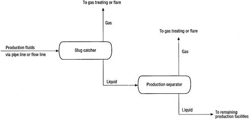
Figure 13-14 Location of Slug Catcher and Production Separator [36]

Figure 13-15 Combined Slug Catcher and Production Separator [36]
13.7.1 Slug Catcher Design Process
The goal of slug catcher design is to properly size the slug catcher for the appropriate conditions. The process consists of the following steps:
13.7.2 Slug Catcher Functions
The slug catcher functions may be summarized as follows:
Each slug catcher can serve one or more functions, and each function is detailed in the following sections.
13.7.2.1 Process Stabilization
Process stabilization is the primary purpose of the slug catcher. In a typical steady-state operation, multiphase production fluids from the flowlines enter the production facilities at constant temperature, pressure, velocity, and flow rate. Process control devices such as pressure control valves and level control valves are used to maintain steady operating conditions throughout the process facilities. During non-steady-state conditions, such as start-up, shutdown, turndown, and pigging, or when slugging during normal operation is expected, the process controllers alone may not be able to sufficiently compensate for the wide variations in fluid flow rates, vessel liquid levels, fluid velocities, and system pressures caused by the slugs.
A slug catcher provides sufficient space to dampen the effects of flow rate surges in order to minimize mechanical damage and deliver an even supply of gas and liquid to the rest of the production facilities, minimizing process and operation upsets.
13.7.2.2 Phase Separation
The second main function of the slug catcher is to provide a means to separate multiphase production fluids into separate gas and liquid streams in order to reduce liquid carryover in the gas stream and gas re-entrainment in the liquid stream. When a slug catcher is provided at the upstream end of a production separator as shown in Figure 13-14, the slug catcher is designed primarily for process stabilization. Gas/liquid separation also occurs, but the efficiency of separation is usually not sufficient to meet oil and gas product specifications. The gas stream may need additional treating to remove entrained liquids prior to treating, compression, or flaring. The liquid may need additional treating for gas/oil/water separation and crude stabilization.
When a separate slug catcher is not provided, the production separator is designed for both process stabilization and efficient gas/liquid separation as shown in Figure 13-15. Production separators, which also function as slug catchers, are generally not designed for gas/oil/water separation. This is because the level surges due to slugging, making it difficult to control the oil/water interface.
13.7.2.3 Storage
Slugs that result from pigging can often be significantly larger than terrain-induced slugs or slugs formed while operating in the slug-flow regime, particularly for gas/condensate systems with long flowlines or pipelines. In these situations, the condensate processing and handling systems may not be sized to quickly process the large slug volume that results from pigging. The slug catcher then acts as a storage vessel to hold the condensate until it can gradually be metered into the process or transported to another location.
13.8 Pressure Surge
13.8.1 Fundamentals of Pressure Surge
An important consideration in the design of single-liquid-phase pipelines is pressure surge, also known as water hammer. Typical surge events in a pipeline or piping system are generally caused by a pump shutdown or a valve closure [37]. The kinetic energy of flow is converted to pressure energy. The velocity of the pressure wave propagation is determined by fluid and pipeline characteristics. Typical propagation velocities range from 1100 ft/s for propane/butane pipelines to 3300 ft/s for crude oil pipelines and up to 4200 ft/s for heavy-wall steel water pipelines.
A rough estimate of the total transient pressure in a pipeline/piping system following a surge event can be obtained from the following equations:
![]() (13-27)
(13-27)
where
vs : speed of sound in the fluid, propagation speed of the pressure wave, ft/s;
K: fluid bulk modulus, 20 ksi;
g: gravitational constant, 32.2 ft/s2;
ρ: density of liquid, lbf/ft3;
d: inside diameter of pipe, in.;
E: pipe material modulus of elasticity, psi;
C: constant of pipe fixity; 0.91 for an axially restrained line; 0.95 for unrestrained.
The surge pressure wave travels upstream and is reflected downstream, oscillating back and forth until its energy is dissipated in pipe wall friction. The amplitude of the surge wave, or the magnitude of the pressure surge Psurge, is a function of the change in velocity and the steepness of the wave front and is the inverse of the time it took to generate the wave:
![]() (13-28)
(13-28)
where
This is only a rough estimation of the surge pressure magnitude for cases limited by the stated time of closure criteria. An accurate analysis of the maximum surge pressure and location of critical points in the system may be obtained from a dynamic simulation by using software such as Pipe Simulator. The surges are attenuated by friction, and the surge arriving at any point on the line is less than at the origin of the surge wave. Nevertheless, when the flow velocity is high and stoppage is complete, or when a pump station is bypassed suddenly, the surge energy generated can produce pressures high enough to burst pipe. Based on the ASME codes, the level of pressure rise due to surges and other variations from normal operations shall not exceed the internal design pressure at any point in the piping system and equipment by more than 10%.
13.8.2 Pressure Surge Analysis
Surge analysis should be performed during a project’s early design and planning phases. This analysis will help to ensure the achievement of an integrated and economical design. Surge analysis provides assurance that the selected pumps/compressors, drivers, control valves, sensors, and piping can function as an integrated system in accordance with a suitable control system philosophy. A surge analysis becomes mandatory when one repairs a ruptured pipeline/piping system to determine the source of the problem.
All long pipelines/piping systems designed for high flow velocities should be checked for possible surge pressures that could exceed the maximum allowable surge pressure (MASP) of the system piping or components. A long pipeline/piping system is defined as one that can experience significant changes in flow velocity within the critical period. By this definition, a long pipeline/piping system may be 1500 ft long or 800 miles long.
A steady-state design cannot properly reflect system operation during a surge event. On one project in which a loading hose at a tanker loading system in the North Sea normally operated at 25 to 50 psig, a motor-operated valve at the tanker manifold malfunctioned and closed during tanker loading. The loading hose, which had a pressure rating of 225 psig, ruptured. Surge pressure simulation showed that the hydraulic transient pressure exceeded 550 psig. Severe surge problems can be mitigated through the use of quick-acting relief valves, tanks, and gas-filled surge bottles, but these facilities are expensive single-purpose devices.
13.9 Line Sizing
13.9.1 Hydraulic Calculations
Hydraulic calculations should be carried out from wells, pipelines, and risers to the surface facilities in line sizing. The control factors in the calculation are fluids (oil, gas, or condensate fluids), flowline size, flow pattern, and application region. Unlike single-phase pipelines, multiphase pipelines are sized taking into account the limitations imposed by production rates, erosion, slugging, and ramp-up speed. Artificial lift is also considered during line sizing to improve the operational range of the system.
Design conditions are as follows:
• Flow rate and pressure drop allowable established: Determine pipe size for a fixed length.
• Flow rate and length known: Determine pressure drop and line size.
Usually either of these conditions requires a trial-and-error approach based on assumed pipe sizes to meet the stated conditions. Some design problems may require determination of maximum flow for a given line size and length, but this is a reverse of the conditions above.
During the FEED stage of a project, the capability of a given line size to deliver the production rate throughout the life of the field is determined by steady-state simulation from the reservoir to the surface facilities throughout the field life. Sensitivities to the important variables such as GOR, water cut, viscosity, and separator pressure should be examined.
The technical criteria for line sizing of pipelines are stated in next section; however, the optimum economic line size is seldom realized in the engineering design. Unknown factors such as future flow rate allowances, actual pressure drops through certain process equipment, etc., can easily overcompensate for what the design predicted when selecting the optimum. In sizing a pipeline, one is always faced with a compromise between two factors. For a given flow rate of a given fluid, piping cost increases with diameter. But pressure loss decreases, which reduces potential pumping or compression costs. There is an economic balance between material costs and pumping costs in downstream flowlines. The optimum pipe size is found by calculating the smallest capitalization/operating cost or using the entire pressure drop available; or increasing velocity to highest allowable.
13.9.2 Criteria
The line sizing of the pipeline is governed by the following technical criteria:
Other criteria considered in the selection of the optimum line size include:
• Standard versus custom line sizes: Generally, standard pipe is less expensive and more readily available. For long pipelines or multiple pipelines for the same size, custom line sizes may be cost effective.
• Ability of installation: Particularly in deep water, the technical installation feasibility of larger line sizes may constrain the maximum pipe size.
• Future production: Consideration should be given to future production that may utilize the lines.
• Number of flowlines and risers: If construction or flow assurance constraints require more than two production flowlines per manifold, optional alternatives including subsea metering processing and bundles should be explored.
• Low-temperature limits: Subsea equipment including trees, jumpers, manifolds, and flowlines have minimum temperature specifications. For systems with Joule-Thompson cooling in low ambient temperature environments, operating philosophies and possibly metallurgical sections should be adjusted.
• High-temperature limits: Flexible pipe has a maximum temperature limit that depends on the materials of construction, water cut, water composition, and water pH. For systems with flexible pipe, the flow rate may be limited, requiring a smaller pipe.
• Roughness: Flexible pipe is rougher than steel pipe and, therefore, requires a larger diameter for the same maximum rate. To smooth flexible pipe, an internal coating may be applied.
13.9.3 Maximum Operating Velocities
Liquid velocity is usually limited because of erosion effects at fittings. Erosion damage can occur in flowlines with multiphase flow because of the continuous impingement of high-velocity liquid droplets. The damage is almost always confined to the place where the flow direction is changed, such as elbows, tees, manifolds, valves, and risers. The erosional velocity is defined as the bulk fluid velocity that will result in the removal of corrosion product scales, corrosion inhibitors, or other protective scales present on the intersurface of a pipeline [38].
The velocity of pipeline fluids should be constrained as follows:
• The fluid velocity in single-phase liquid lines varies from 0.9 to 4.5 m/s (3 to 15 ft/s).
• Gas/liquid two-phase lines do not exceed the erosional velocity as determined from following equation, which is recommended in API RP 14E [39]:
![]() (13-29)
(13-29)
where
Vmax: maximum allowable mixture erosional velocity, m/s (ft/s);
ρ: density of the gas/liquid mixture, kg/m3 (lb/ft3);
C: empirical constant, which determined in Table 13-9.
Table 13-9. Empirical Constant in the Equation
| Service Type | Operational Frequency | |
| Continuous | Intermittent | |
| Two-phase flow without sand | 100 | 125 |
| If possible, the minimum velocity in two-phase lines should be greater than 3 m/s (10 ft/s) to minimize slugging. | ||
The mixture density, ρm is defined as:
![]() (13-30)
(13-30)
where
Assuming on erosion rate of 10 mils per year, the following maximum allowable velocity is recommended by Salama and Venkatesh [40], when sand appears in an oil/gas mixture flow:
![]() (13-31)
(13-31)
where
Erosion limits or maximum velocities for flexible pipes should be specified by the manufacturer. The API erosion velocity limit is normally very conservative and the practice of this limit could vary depend on different operators.
13.9.4 Minimum Operating Velocities
The following items may effectively impose minimum velocity constraints:
• Slugging: Slugging severity typically increases with decreasing flow rate. The minimum allowable velocity constraint should be imposed to control the slugging in multiphase flow for assuring the production deliverability of the system.
• Liquid handling: In gas/condensate systems, the ramp-up rates may be limited by the liquid handling facilities and constrained by the maximum line size.
• Pressure drop: For viscous oils, a minimum flow rate is necessary to maintain fluid temperature such that the viscosities are acceptable. Below this minimum, production may eventually shut itself in.
• Liquid loading: A minimum velocity is required to lift the liquids and prevent wells and risers from loading up with liquid and shutting in. The minimum stable rate is determined by transient simulation at successively lower flow rates. The minimum rate for the system is also a function of GLR.
• Sand bedding: The minimum velocity is required to avoid sand bedding.
13.9.5 Wells
During FEED analysis, the production system should be modeled starting at the reservoir using inflow performance relationships. OLGA 2000 may be used to evaluate the hydraulic stability of the entire system including the wells, flowlines, and risers subject to artificial lift to get minimum stable rates as a function of the operating requirements and artificial lift.
In the hydraulic and thermal analyses of subsea flowline systems, the wellhead pressure and temperature are generally used as the inlet pressure and temperature of the system. The wellhead pressure and temperature are functions of reservoir pressure, temperature, productivity index, and production rate and can be obtained from steady and transient hydraulic and thermal analyses of the well bore. The hydraulic and thermal models may be simulated using the commercial software PIPESIM or OLGA 2000.
The hydraulic and thermal processes of a wellbore are simulated for the following purposes:
• Determining steady-state wellhead pressure and temperature for flowline hydraulics and thermal analyses.
• Determining the minimum production rates that will prevent hydrate formation in the wellbore.
• Determining the minimum production rate for preventing wax deposition in the wellbore and tree. The wellhead temperature is required to be higher than the critical wax deposition temperature in the steady-state flowing condition.
• Determining cooldown time and warm-up time from transient wellbore analysis to prevent hydrate formation in the wellbore.
The transient analyses determine how hydrates can be controlled during startup and shut-in processes. Vacuum insulated tubing (VIT) is one method to help a wellbore out of the hydrate region. Use of 3000 to 4000 ft of VIT results in warm-up of the wellbore to temperatures above the hydrate temperature in typically 2 hr or less. These warm-up rates are rapid enough to ensure that little or no hydrates form in the wellbore. This makes it possible to eliminate the downhole injection of methanol above the subsurface safety valve during warm-up. Instead, methanol is injected upstream of the choke to prevent any hydrates that may be formed during warm-up from plugging the choke. One drawback of VIT is that it cools more quickly than bare tubing since the insulation prevents the tubing from gaining heat from the earth, which also warms up during production. As a result of this quick cooling, it is necessary to quickly treat the wellbore with methanol in the event that a production shut-in occurs during the warm-up period. For a higher reservoir temperature, VIT may not be used in the wellbore, and the cooldown speed of a wellbore is very slow after a process interruption from steady-state production conditions.
13.9.6 Gas Lift
Artificial lift can be used to increase production rates or reduce line sizes. Line sizing may include the affects of gas lift.
For systems employing gas lift, models should extend from the reservoir to the surface facilities incorporating the gas lift gas in addition to the produced fluids. The composition of the gas-lift gas is provided by the topside process but should meet the dew-point control requirement. The preferred location (downhole, flowline inlet, or riser base) is determined based on effectiveness and cost.
The effect of gas lift on the severe slugging boundary may be simulated with OLGA 2000 for the situations, when it is required. Normally, it is set at the riser base. The simulation may decide the minimum flow rate without severe slugging as a function of gas-lift rates and water cuts. When the gas-lift injection point does not include a restriction or valve to choke the gas flows, OLGA 2000 transient simulations may model the transient flow in the gas-lift line by including the gas-lift line as a separate branch to determine maximum variation in mass rate and pressure and still maintain system stability. Maximum production rates throughout the field life are determined as a function of gas-lift rate. In FEED designs, the gas-lift rate and pressure requirements should be recommended, including a measurement and control strategy for the gas-lift system.
REFERENCES
1. Reid RC, Prausnitz JM, Sherwood TK. The Properties of Gases and Liquids. third ed. New York: McGraw-Hill; 1977.
2. Pedersen KS, Fredenslund A, Thomassen P. Properties of Oils and Natural Gases. Gulf Publishing Company 1989.
3. Leland TW, Phase Equilibria, Fluid. Properties in the Chemical Industry. Frankfurt/Main: DECHEMA; 1980; 283–333.
4. Soave G. Equilibrium Constants from a Modified Redilich-Kwong Equation of State. Chem Eng Sci. 1972;vol. 27:1197–1203.
5. Peng DY, Robinson DB. A New Two-Constant Equation of State. Ind Eng Chem Fundam. 1976;vol. 15:59–64.
6. Gregory GA. Viscosity of Heavy Oil/Condensate Blends, Technical Note, No 6. Calgary, Canada: Neotechnology Consultants Ltd; 1985.
7. Gregory GA. Pipeline Calculations for Foaming Crude Oils and Crude Oil-Water Emulsions, Technical Note No 11. Calgary, Canada: Neotechnology Consultants Ltd; 1990.
8. Woelflin W. The Viscosity of Crude Oil Emulsions, in Drill and Production Practice. American Petroleum Institute. 1942;vol. 148:p247.
9. Guth E, Simha R. Untersuchungen über die Viskosität von Suspensionen und Lösungen 3 Über die Viskosität von Kugelsuspensionen. Kolloid-Zeitschrift. 1936;vol. 74:266–275.
10. Smith HV, Arnold KE. Crude Oil Emulsions, in Petroleum Engineering Handbook. In: Bradley HB, ed. Richardson, Texas: Society of Petroleum Engineers; 1987.
11. C.H. Whitson, M.R. Brule, Phase Behavior, Monograph 20, Henry, L. Doherty Series, Society of Petroleum Engineers, Richardson, Texas, (2000).
12. Mohinder LN, ed. Piping Handbook. New York: McGraw-Hill; 1999.
13. Moody LF. Friction Factors for Pipe Flow, Trans. ASME. 1944;vol. 66:671–678.
14. Larock BE, Jeppson RW, Watters GZ. Hydraulics of Pipeline Systems. Boca Raton, Florida: CRC Press; 1999.
15. Crane Company, Flow of Fluids through Valves, Fittings and Pipe, Technical Paper No. 410, 25th printing, (1991).
16. J.P. Brill, H. Mukherjee, Multiphase Flow in Wells, Monograph vol. 17(1999), L. Henry, Doherty Series, Society of Petroleum Engineers, Richardson, Texas.
17. Beggs HD, Brill JP. A Study of Two Phase Flow in Inclined Pipes. Journal of Petroleum Technology. 1973;vol. 25(No. 5):607–617.
18. Taitel YM, Barnea D, Dukler AE. Modeling Flow Pattern Transitions for Steady Upward Gas-Liquid Flow in Vertical Tubes. AIChE Journal. 1980;vol. 26:245.
19. PIPESIM Course, Information on Flow Correlations used within PIPESIM, (1997).
20. Duns H, Ros NCJ. Vertical Flow of Gas and Liquid Mixtures in Wells. Frankfurt: Proc. 6th World Petroleum Congress, Section II, Paper 22-106; 1963.
21. Qrkifizewski J. Predicting Two-Phase Pressure Drops in Vertical Pipes. Journal of Petroleum Technology 1967:829–838.
22. Hagedom AR, Brown KE. Experimental Study of Pressure Gradients Occurring During Continuous Two-Phase Flow in Small-Diameter Vertical Conduits. Journal of Petroleum Technology 1965:475–484.
23. Mukherjce H, Brill JP. Liquid Holdup Correlations for Inclined Two-Phase Flow. Journal of Petroleum Technology 1983:1003–1008.
24. Aziz KL, Govier GW, Fogarasi M. Pressure Drop in Wells Producing Oil and Gas. Journal of Canadian Petroleum Technology. 1972;vol. 11:38–48.
25. Beniksen KH, Malnes D, Moe R, Nuland S. The Dynamic Two-Fluid Model OLGA: Theory and Application. SPE Production Engineering. 1991;6:171–180 SPE 19451.
26. Ansari A, Sylvester ND, Shoham O, Brill JP. A Comprehensive Mechanistic Model for Upward Two-Phase Flow in Wellbores. SPE 20630, SPE Annual Technical Conference 1990.
27. Baker AC, Nielsen K, Gabb A. Pressure Loss, Liquid-holdup Calculations Developed. Oil & Gas Journal. 1988;vol. 86(No 11):55–59.
28. Flanigan O. Effect of Uphill Flow on Pressure Drop in Design of Two-Phase Gathering Systems. Oil & Gas Journal. 1958;vol. 56:132–141.
29. Dukler EA, et al. Gas-Liquid Flow in Pipelines. I Research Results, AGA-API Project NX-28 1969.
30. R.V.A. Oliemana, Two-Phase Flow in Gas-Transmission Pipeline, ASME paper 76-Pet-25, presented at Petroleum Division ASME Meeting, Mexico City, (1976).
31. W.G. Gray, Vertical Flow Correlation Gas Wells API Manual 14BM (1978).
32. J.J. Xiao, O. Shoham, J.P. Brill, A Comprehensive Mechanistic Model for Two-Phase Flow in Pipelines, SPE, (1990). SPE 20631.
33. Fayed SF, Otten L. Comparing Measured with Calculated Multiphase Flow Pressure Drop. Oil & Gas Journal. 1983;vol. 6:136–144.
34. Feesa Ltd, Hydrodynamic Slug Size in Multiphase Flowlines, retrieved from http://www. feesa.net/flowassurance.(2003).
35. Scandpower, OLGA 2000, OLGA School, Level I, II.
36. Deepstar, Flow Assurance Design Guideline, Deepstar IV Project, DSIV CTR 4203b–1, (2001).
37. Wu JC. Benefits of Dynamic Simulation of Piping and Pipelines. Paragon Technotes 2001.
38. Gregory GA. Erosional Velocity Limitations for Oil and Gas Wells, Technical Note No 5. Calgary, Canada: Neotechnology Consultants Ltd; 1991.
39. American Petroleum Institute. Recommended Practice for Design and Installation of Offshore Platform Piping System. fifth edition API RP 14E 1991.
40. Salama MM, Venkatesh ES. Evaluation of API RP 14E Erosional Velocity Limitations for Offshore Gas Wells. OTC. 1983;4485.