
“The only certainty is uncertainty.”
— Pliny the Elder
The future has uncertainty for sure. The best we can do is plan for it. And for meticulous planning, we need to have a peek into the future. If we can know beforehand how much the expected demand for our product is, we will manufacture adequately—not more, not less. We will also rectify the bottlenecks in our supply chain if we know what the expected traffic of goods is. Airports can plan resources better if they know the expected inflow of passengers. Or ecommerce portals can plan for the expected load if they know how many clicks are expected during the upcoming sale season.
It may not be possible to forecast accurately, but it is indeed required to predict these values. It is still done, with or without ML-based predictive modeling, for financial budget planning, allocation of resources, guidance issued, expected rate of growth, and so on. Hence, the estimation of such values is of paramount importance. In this second chapter, we will be studying the precise concepts to predict such values.
In the first chapter, we introduced supervised learning. The differentiation between supervised, unsupervised, and semi-supervised was also discussed. We also examined the two types of supervised algorithms: regression and classification. In this second chapter, we will study and develop deeper concepts of supervised regression algorithms.
We will be examining the regression process, how a model is trained, behind-the-scenes process, and finally the execution for all the algorithms. The assumptions for the algorithms, the pros and cons, and statistical background beneath each one will be studied. We will also develop code in Python using the algorithms. The steps in data preparation, data preprocessing, variable creation, train-test split, fitting the ML model, getting significant variables, and measuring the accuracy will all be studied and developed using Python. The codes and datasets are uploaded to a GitHub repository for easy access. You are advised to replicate those codes yourself.
Technical Toolkit Required
We are going to use Python 3.5 or above in this book. You are advised to get Python installed on your machine. We will be using Jupyter notebook; installing Anaconda-Navigator is required for executing the codes. All the datasets and codes have been uploaded to the Github repository at https://github.com/Apress/supervised-learning-w-python/tree/master/Chapter2 for easy download and execution.
The major libraries used are numpy, pandas, matplotlib, seaborn, scikit learn, and so on. You are advised to install these libraries in your Python environment.
Let us go into the regression analysis and examine the concepts in detail!
Regression analysis and Use Cases
Regression analysis is used to estimate the value of a continuous variable. Recall that a continuous variable is a variable which can take any numerical value; for example, sales, amount of rainfall, number of customers, number of transactions, and so on. If we want to estimate the sales for the next month or the number of passengers expected to visit the terminal in the next week or the number of customers expected to make bank transactions, we use regression analysis.
Simply put, if we want to predict the value of a continuous variable using supervised learning algorithms, we use regression methods. Regression analysis is quite central to business solving and decision making. The predicted values help the stakeholders allocate resources accordingly and plan for the expected increase/decrease in the business.
- 1.
A retailer wants to estimate the number of customers it can expect in the upcoming sale season. Based on the estimation, the business can plan on the inventory of goods, number of staff required, resources required, and so on to be able to cater to the demand. Regression algorithms can help in that estimation.
- 2.
A manufacturing plant is doing a yearly budget planning. As a part of the exercise, expenditures under various headings like electricity, water, raw material, human resources, and so on have to be estimated in relation to the expected demand. Regression algorithms can help assess historical data and generate estimates for the business.
- 3.
A real estate agency wishes to increase its customer base. One important attribute is the price of the apartments, which can be improved and generated judiciously. The agency wants to analyze multiple parameters which impact the price of property, and this can be achieved by regression analysis.
- 4.
An international airport wishes to improve the planning and gauge the expected traffic in the next month. This will allow the team to maintain the best service quality. Regression analysis can help in that and make an estimation of the number of estimated passengers.
- 5.
A bank which offers credit cards to its customers has to identify how much credit should be offered to a new customer. Based on customer details like age, occupation, monthly salary, expenditure, historical records, and so on, a credit limit has to be prescribed. Supervised regression algorithms will be helpful in that decision.
- 1.
Linear regression
- 2.
Decision tree
- 3.
Random forest
- 4.
SVM
- 5.
Bayesian methods
- 6.
Neural networks
We will study the first three algorithms in this chapter and the rest in Chapter 4. We are starting with linear regression in the next section.
What Is Linear Regression

(i) The data in a vector-space diagram depicts how price is dependent on various variables. (ii) An ML regression equation called the line of best fit is used to model the relationship here, which can be used for making future predictions for the unseen dataset.
Correlation analysis is used to measure the strength of association (linear relationship) between two variables.
If two variables move together in the same direction, they are positively correlated. For example: height and weight will have a positive relationship. If the two variables move in the opposite direction, they are negatively correlated. For example, cost and profit are negatively related.
The range of correlation coefficient ranges from –1 to +1. If the value is –1, it is absolute negative correlation; if it is +1, correlation is absolute positive.
If the correlation is 0, it means there is not much of a relationship. For example, the price of shoes and computers will have low correlation.
The objective of the linear regression analysis is to measure this relationship and arrive at a mathematical equation for the relationship. The relationship can be used to predict the values for unseen data points. For example, in the case of the house price problem, predicting the price of a house will be the objective of the analysis.
Formally put, linear regression is used to predict the value of a dependent variable based on the values of at least one independent variable. It also explains the impact of changes in an independent variable on the dependent variable. The dependent variable is also called the target variable or endogenous variable. The independent variable is also termed the explanatory variable or exogenous variable.
Linear regression has been in existence for a long time. Though there are quite a few advanced algorithms (some of which we are discussing in later chapters), still linear regression is widely used. It serves as a benchmark model and generally is the first step to study supervised learning. You are advised to understand and examine linear regression closely before you graduate to higher-degree algorithms.

where
Yi = Dependent variable or the target variable which we want to predict
xi = Independent variable or the predicting variables used to predict the value of Y
β0 = Population Y intercept. It represents the value of Y when the value of xi is zero
β1 = Population slope coefficient. It represents the expected change in the value of Y by a unit change in xi
ε = random error term in the model
Sometimes, β0 and β1 are called the population model coefficients.

A linear regression equation depicted on a graph showing the intercept, slope, and actual and predicted values for the target variable; the red line shows the line of best fit
These model coefficients (β0 and β1) have an important role to play. Y intercept (β0) is the value of dependent variable when the value of independent variable is 0, that is, it is the default value of dependent variable. Slope (β1) is the slope of the equation. It is the change expected in the value of Y with unit change in the value of x. It measures the impact of x on the value of Y. The higher the absolute value of (β1), the higher is the final impact.
Figure 2-2 also shows the predicted values. We can understand that for the value of x for observation i, the actual value of dependent variable is Yi and the predicted value or estimated value is  .
.
There is one more term here, random error
, which is represented by ε. After we have made the estimates, we would like to know how we have done, that is, how far the predicted value is from the actual value. It is represented by random error, which is the difference between the predicted and actual value of Y and is given by  . It is important to note that the smaller the value of this error, the better is the prediction.

(i) The data in a vector-space diagram depicts how price is dependent on various variables. (ii) While trying to model for the data, there can be multiple linear equations which can fit, but the objective will be to find the equation which gives the minimum loss for the data at hand.
Hence, it turns out that we have to find out the best mathematical equation which can minimize the random error and hence can be used for making the predictions. This is achieved during training of the regression algorithm. During the process of training the linear regression model, we get the values of β0 and β1, which will minimize the error and can be used to generate the predictions for us.
The linear regression model makes some assumptions about the data that is being used. These conditions are a litmus test to check if the data we are analyzing follows the requirements or not. More often, data is not conforming to the assumptions and hence we have to take corrective measures to make it better. These assumptions will be discussed now.
Assumptions of Linear Regression
- 1.Linear regression needs the relationship between dependent and independent variables to be linear. It is also important to check for outliers since linear regression is sensitive to outliers. The linearity assumption can best be tested with scatter plots. In Figure 2-4, we can see the meaning of linearity vs. nonlinearity. The figure on the left has a somewhat linear relationship where the one on the right does not have a linear relationship.
 Figure 2-4
(i) There is a linear relationship between X and Y. (ii) There is not much of a relationship between X and Y variables; in such a case it will be difficult to model the relationship.
- 2.
Linear regression requires all the independent variables to be multivariate normal. This assumption can be tested using a histogram or a Q-Q plot. The normality can be checked with a goodness-of-fit test like the Kolmogorov-Smirnov test. If the data is not normally distributed, a nonlinear transformation like log transformation can help fix the issue.
- 3.The third assumption is that there is little or no multicollinearity in the data. When the independent variables are highly correlated with each other, it gives rise to multicollinearity. Multicollinearity can be tested using three methods:
- a.
Correlation matrix: In this method, we measure Pearson’s bivariate correlation coefficient between all the independent variables. The closer the value to 1 or –1, the higher is the correlation.
- b.
Tolerance: Tolerance is derived during the regression analysis only and measures how one independent variable is impacting other independent variables. It is represented as (1 – R2). We are discussing R2 in the next section If the value of tolerance is < 0.1, there are chances of multicollinearity present in the data. If it is less than 0.01, then we are sure that multicollinearity is indeed present.
- c.
Variance Inflation Factor (VIF) : VIF can be defined as the inverse of tolerance (1/T). If the value of VIF is greater than 10, there are chances of multicollinearity present in the data. If it is greater than 100, then we are sure that multicollinearity is indeed present.
Note Centering the data (deducting mean from each score) helps to solve the problem of multicollinearity. We will examine this in detail in Chapter 5!
- a.
- 4.
Linear regression assumes that there is little or no autocorrelation present in the data. Autocorrelation means that the residuals are not independent of each other. The best example for autocorrelated data is in a time series data like stock prices. The prices of stock on Tn+1 are dependent on Tn. While we use a scatter plot to check for the autocorrelation, we can use Durbin-Watson’s “d-test” to check for the autocorrelation. Its null hypothesis is that the residuals are not autocorrelated. If the value of d is around 2, it means there is no autocorrelation. Generally d can take any value between 0 and 4, but as a rule of thumb 1.5 < d < 2.5 means there is no autocorrelation present in the data. But there is a catch in the Durbin-Watson test. Since it analyzes only linear autocorrelation and between direct neighbors only, many times, scatter plot serves the purpose for us.
- 5.
The last assumption in a linear regression problem is homoscedasticity, which means that the residuals are equal over the regression line. While a scatter plot can be used to check for homoscedasticity, the Goldfeld-Quandt test can also be used for heteroscedasticity. This test divides the data into two groups. Then it tests if the variance of residuals is similar across the two groups. Figure 2-5 shows an example of residuals which are not homoscedastic. In such a case, we can do a nonlinear correction to fix the problem. As we can see in Figure 2-5, heteroscedasticity results in a distinctive cone shape in the residual plots.

Heteroscedasticity is present in the dataset and hence there is a cone-like shape in the residual scatter plot
These assumptions are vital to be tested and more often we transform our data and clean it. It is imperative since we want our solution to work very well and have a good prediction accuracy. An accurate ML model will have a low loss. This accuracy measurement process for an ML model is based on the target variable. It is different for classification and regression problems. In this chapter, we are discussing regression base models while in the next chapter we will examine the classification model’s accuracy measurement parameters. That brings us to the important topic of measuring the accuracy of a regression problem, which is the next topic of discussion.
Measuring the Efficacy of Regression Problem
 , which are nothing but the actual and predicted values of the dependent variable as shown in Figure 2-6. This is referred to as the loss function, which means the loss incurred in making a prediction. Needless to say, we want to minimize this loss to get the best model. The errors are referred as residuals too.
The difference between the actual values and predicted values of the target variable. This is the error made while making the prediction, and as a best model, this error is to be minimized.
A very important point: why do we take a square of the errors? The reason is that if we do not take the squares of the errors, the positive and negative terms can cancel each other. For example, if the error1 is +2 and error2 is -2, then net error will be 0!


A point to be noted is that the regression line always passes through the mean  and
and ![]() .
.

Where ![]() : Average value of dependent variable
: Average value of dependent variable
Yi: Observed value of the dependent variable
![]() : Predicted value of y for the given value of xi
: Predicted value of y for the given value of xi
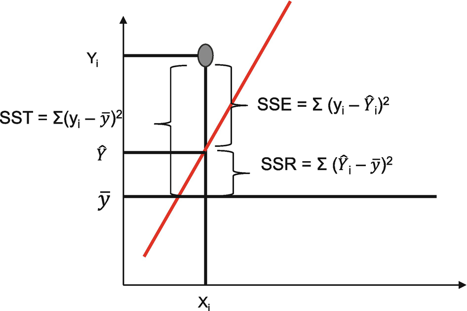
SST = Total sum of squares: SSE = Error sum of squares, and SSR = Regression sum of squares
- 1.
Mean absolute error (MAE): As the name suggests, it is the average of the absolute difference between the actual and predicted values of a target variable as shown in Equation 2-5.

- 2.
Mean squared error (MSE): MSE is the average of the square of the error, that is, the difference between the actual and predicted values as shown in Equation 2-6. Similar to MAE, a higher value of MSE means higher error in our model.

- 3.
Root MSE: Root MSE is the square root of the average squared error and is represented by Equation 2-7.

- 4.
R square (R2): It represents how much randomness in the data is being explained by our model. In other words, out of the total variation in our data how much is our model able to decipher.
R2 = SSR/SST = Regression sum of squares/Total sum or squares
R2 will always be between 0 and 1 or 0% and 100%. The higher the value of R2, the better it is. The way to visualize R2 is depicted in the following figures. In Figure 2-8, the value of R2 is equal to 1, which means 100% of the variation in the value of Y is explainable by x. In Figure 2-9, the value of R2 is between 0 and 1, depicting that some of the variation is understood by the model. In the last case, Figure 2-9, R2 = 0, which shows that no variation is understood by the model. In a normal business scenario, we get R2 between 0 and 1, that is, a portion of the variation is explained by the model. Figure 2-8
R2 is equal to 1; this shows that 100% of the variation in the values of the independent variable is explained by our regression model
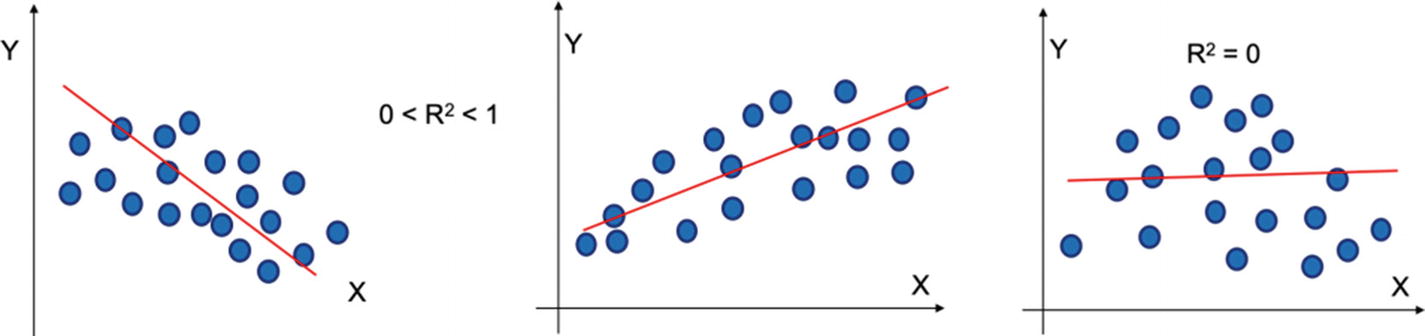 Figure 2-9
If the value of R2 is between 0 and 1 then partial variation is explained by the model. If the value is 0, then no variation is explained by the regression model
- 5.
Pseudo R square : It extends the concept of R square. It penalizes the value if we include insignificant variables in the model. We can calculate pseudo R2 as in Equation 2-8.

where n is the sample size and k is the number of independent variables
Using R square, we measure all the randomness explained in the model. But if we include all the independent variables including insignificant ones, we cannot claim that the model is robust. Hence, we can say pseudo R square is a better representation and measure to measure the robustness of a model.
Between R2 and pseudo R2, we prefer pseudo R2. The higher the value, the better the model.
Now we are clear on the assumptions of a regression model and how we can measure the performance of a regression model. Now let us study types of linear regression and then develop a Python solution.
Linear regression can be studied in two formats: simple linear regression and multiple linear regression.
Square feet (x) | Price (in 1000 $) |
|---|---|
1200 | 100 |
1500 | 120 |
1600 | 125 |
1100 | 95 |
1500 | 125 |
2200 | 200 |
2100 | 195 |
1410 | 110 |
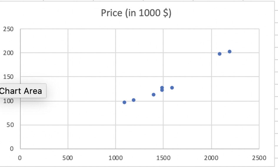
Scatter plot of the price and area data

Here price is Y (dependent variable) and area is the x variable (independent variable). The goal of the simple linear regression will be to estimate the values of β0 and β1 so that we can predict the values of price.
- 1.
β0 having a value of –28.07 means that when the square footage is 0 then the price is –$28,070. Now it is not possible to have a house with 0 area; it just indicates that for houses within the range of sizes observed, $28,070 is the portion of the house price not explained by the area.
- 2.
β1 is 0.10;it indicates that the average value of a house increases by a 0.1 × (1000) = $100 with on average for each additional increase in the size by one square foot.
There is an important limitation to linear regression. We cannot use it to make predictions beyond the limit of the variables we have used in training. For example, in the preceding data set we cannot model to predict the house prices for areas above 2200 square feet and below 1100 square feet. This is because we have not trained the model for such values. Hence, the model is good enough for the values between the minimum and maximum limits only; in the preceding example the valid range is 1100 square feet to 2200 square feet.
- Common hyperparameters
fit_interceprt: if we want to calculate intercept for the model, and it is not required if data is centered
normalize - X will be normalized by subtracting mean & dividing by standard deviation
By standardizing data before subjecting to model, coefficients tell the importance of features
- Common attributes
coefficients are the weights for each independent variable
intercept is the bias of independent term of linear models
- Common functions
fit - trains the model. Takes X & Y as the input value and trains the model
predict - once model is trained, for given X using predict function Y can be predicted
- Training model
X should be in rows of data format, X.ndim == 2
Y should be 1D for single target & 2D for more than one target
fit function is used for training the model
We will be creating two examples for simple linear regression. In the first example, we are going to generate a simple linear regression problem. Then in example 2, simple linear regression problem will be solved. Let us proceed to example 1 now.
Example 1: Creating a Simple Linear Regression
We are going to create a simple linear regression by generating a dataset. This code snippet is only a warm-up exercise and will familiarize you with the simplest form of simple linear regression.
In the preceding code, n_features is the number of features we want to have in the dataset. n_samples is the number of samples we want to generate. Noise is the standard deviation of the gaussian noise which gets applied to the output.
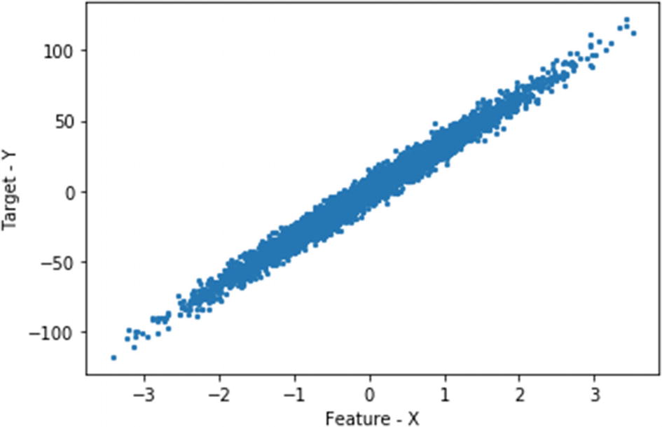
The value for the intercept is 0.6759344 and slope is 33.1810

Blue dots represent maps to actual target data while orange dots represent the predicted values.
We can see that how close the training and actual predicted values are. Now, we will create a solution for simple linear regression using a dataset.
Example 2: Simple Linear Regression for Housing Dataset
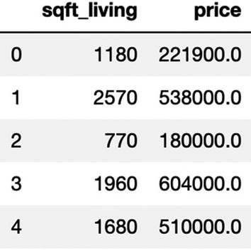
We have a dataset which has one independent variable (area in square feet), and we have to predict the prices. It is again an example of simple linear regression, that is, we have one input variable. The code and dataset are uploaded to the Github link shared at the start of this chapter.
It is a possibility that data is present in the form of .xls or .txt file. Sometimes, the data is to be loaded from the database directly by making a connection to the database.

Step 7: The data is split into train and test now.
Train/Test Split: Creating a train and test dataset involves splitting the dataset into training and testing sets respectively, which are mutually exclusive. After which, you train with the training set and test with the testing set. This will provide a more accurate evaluation of out-of-sample accuracy because the testing dataset is not part of the dataset that has been used to train the data. It is more realistic for real-world problems.
This means that we know the outcome of each data point in this dataset, making it great to test with! And since this data has not been used to train the model, the model has no knowledge of the outcome of these data points. So, in essence, it is truly an out-of-sample testing. Here test data is 25% or 0.25.


In the preceding two examples, we saw how we can use simple linear regression to train a model and make a prediction. In real-world problems, only one independent variable will almost never happen. Most business world problems have more than one variable, and such problems are solved using multiple linear regression algorithms which we are discussing now.
Square Feet | No of bedrooms | Price (in 1000 $) |
|---|---|---|
1200 | 2 | 100 |
1500 | 3 | 120 |
1600 | 3 | 125 |
1100 | 2 | 95 |
1500 | 2 | 125 |
2200 | 4 | 200 |
2100 | 4 | 195 |
1410 | 2 | 110 |

Multiple regression model depiction in vector-space diagram where we have two independent variables, x1 and x2

Hence in the case of a multiple training of the simple linear regression, we will get an estimated value for β0 and β1 and so on.

The multiple linear regression model depicted by x1 and x2 and the residual shown with respect to a sample observation. The residual is the difference between actual and predicted values.
We will now create two example cases using multiple linear regression models. During the model development, we are going to do EDA, which is the first step and will also resolve the problem of null values in the data and how to handle categorical variables too.
Example 3: Multiple Linear Regression for Housing Dataset
We are working on the house price dataset. The target variable is the prediction of house prices and there are some independent variables. The dataset and the codes are uploaded to the Github link shared at the start of this chapter.
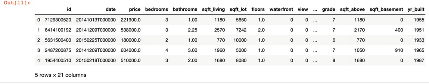
We have 21 variables in this dataset.
Step 3: Next let’s explore the dataset we have. This is done using the house_mlr.info() command.
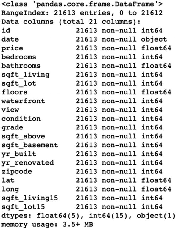
By analyzing the output we can see that out of the 21 variables, there are a few float variables, some object and some integers. We will be treating these categorical variables to integer variables.
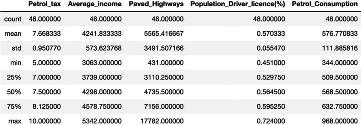
Step 4: house_mlr.describe() command will give the details about all the numeric variables.
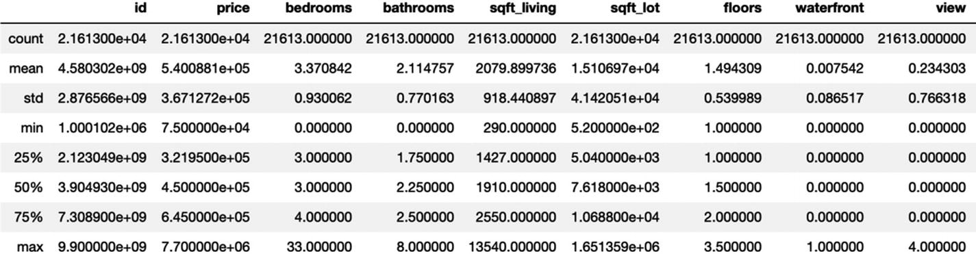
Here we can see the range for all the numeric variables: the mean, standard deviation, the values at the 25th percentile, 50th percentile, and 75th percentile. The minimum and maximum values are also shown.
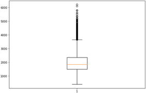
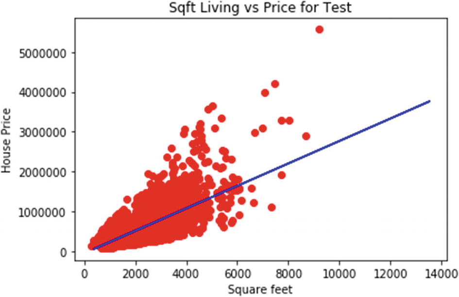
The plot shows that there are a few outliers. In this case, we are not treating the outliers. In later chapters, we shall examine the best practices to deal with outliers.
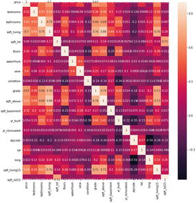
The analysis of the correlation matrix shows that there is some correlation between a few variables. For example, between sqft_above and sqft_living there is a correlation of 0.88. And that is quite expected. For this first simple example, we are not treating the correlated variables.
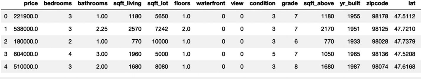
Step 7: The categorical variables are converted to numeric ones using one-hot encoding.
One-hot encoding converts categorical variables to numeric ones. Simply put, it adds new columns to the dataset with 0 or assigned depending on the value of the categorical variable, as shown in the following:


The output we receive is (147274.98522602883, 0.8366403242154088, 0.8358351477235848).
The steps used in this example can be extended to any example where we want to predict a continuous variable. In this problem, we have predicted the value of a continuous variable but we have not selected the significant variables from the list of available variables. Significant variables are the ones which are more important than other independent variables in making the predictions. There are multiple ways to shortlist the variables. We will discuss one of them using the ensemble technique in the next section. The popular methodology of using p-value is discussed in Chapter 3.
With this, we have discussed the concepts and implementation using linear regression. So far, we have assumed that the relationship between dependent and independent variables is linear. But what if this relation is not linear? That is our next topic: nonlinear regression.
Nonlinear Regression Analysis
Consider this. In physics, we have laws of motion to describe the relationship between a body and all the forces acting upon it and how the motion responds to those forces. In one of the laws, the relationship of initial and final velocity is given by the following equation:
Final velocity = initial velocity + ½ acceleration*time2 OR v = u + ½ at2
If we analyze this equation, we can see that the relation between final velocity and time is not linear but quadratic in nature. Nonlinear regression is used to model such relationships. We can review the scatter plot to identify if the relationship is nonlinear as shown in Figure 2-13.
Formally put, if the relationship between target variable and independent variables is not linear in nature, then nonlinear regression is used to fit the data.

Where β0: Y intercept
β1: regression coefficient for linear effect of X on Y
β2 = regression coefficient for quadratic effect on Y and so on
εi = random error in Y for observation i

A nonlinear regression will do a better job to model the data set than a simple linear model. There is no linear relationship between the dependent and the independent variable

Where β0: Y intercept
β1: regression coefficient for linear effect of X on Y
β2 = regression coefficient for quadratic effect on Y
εi = random error in Y for observation i
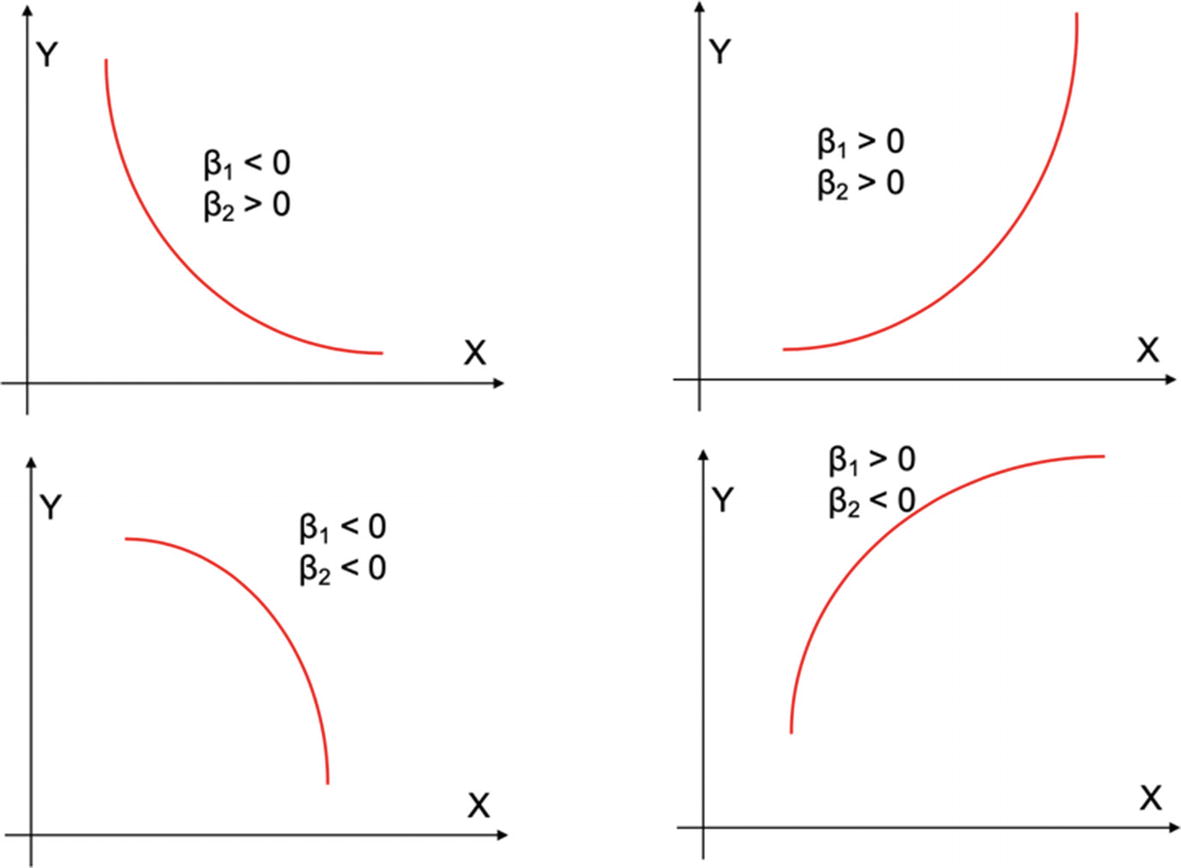
The value of the curve is dependent on the values of β1 and β2. The figure depicts the different shapes of the curve in different directions.
Velocity | Distance |
|---|---|
3 | 9 |
4 | 15 |
5 | 28 |
6 | 38 |
7 | 45 |
8 | 69 |
10 | 96 |
12 | 155 |
18 | 260 |
20 | 410 |
25 | 650 |
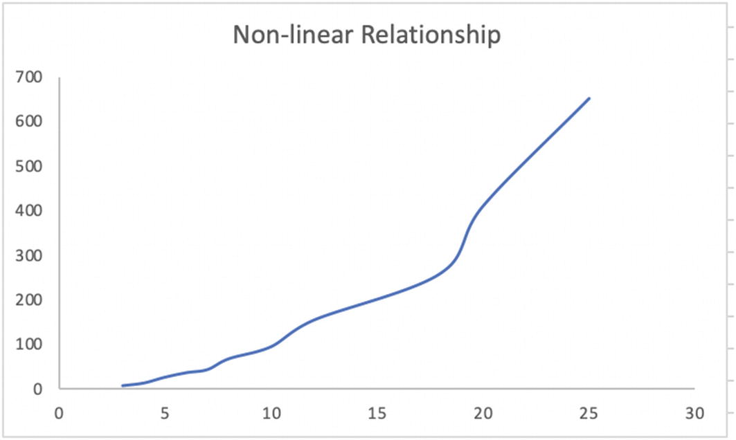
Nonlinear relationship between velocity and distance is depicted here
The data and the respective plot of the data indicate nonlinear relationships. Still, we should know how to detect if a relationship between target and independent variables is nonlinear, which we are discussing next.
Identifying a Nonlinear Relationship
- 1.
The estimate in the case of linear regression is ŷ = b0 + b1x1
- 2.
The estimate in the case of quadratic regression is
 = b0 + b1x1 + b2x21
 - 3.The NULL hypothesis will be
- a.
H0 : β2 = 0 (the quadratic term does not improve the model)
- b.
H1 : β2 ≠ 0 (the quadratic term improves the model)
- a.
- 4.
Once we run the statistical test, we will either accept or reject the NULL hypothesis
- 1.To identify the nonlinear relationship, we can analyze the residuals after fitting a linear model. If we try to fit a linear relationship while the actual relationship is nonlinear, then the residuals will not be random but will have a pattern, as shown in Figure 2-16. If a nonlinear relationship is modeled instead, the residuals will be random in nature.
 Figure 2-16
If the residuals follow a pattern, it signifies that there can be a nonlinear relationship present in the data which is being modeled using a linear model. Linear fit does not give random residuals, while nonlinear fit will give random residuals.
- 2.
We can also compare the respective R2 values of both the linear and nonlinear regression model. If the R2 of the nonlinear model is more, it means the relationship with nonlinear model is better.
Similar to linear regression, nonlinear models too have some assumptions, which we will discuss now.
Assumptions for a Nonlinear Regression
- 1.
The errors in a nonlinear regression follow a normal distribution. Error is the difference between the actual and predicted values and nonlinear requires the variables to follow a normal distribution.
- 2.
All the errors must have a constant variance.
- 3.
The errors are independent of each other and do not follow a pattern. This is a very important assumption since if the errors are not independent of each other, it means that there is still some information in the model equation which we have not extracted.


The coefficient of the independent variable can be interpreted as follows: a 1% change in the independent variable X1 leads to an estimated β1 percentage change in the average value of Y.
Sometimes, β1 can also refer to elasticity of Y with respect to change in X1.
We have studied different types of regression models. It is one of the most stable solutions, but like any other tool or solution, there are a few pitfalls with regression models too. Some of those in the form of important insights will be uncovered while doing EDA. These challenges have to be dealt with while we are doing the data preparation for our statistical modeling . We will now discuss these challenges.
Challenges with a Regression Model
- 1.Nonlinearities : Real-world data points are much more complex and generally do not follow a linear relationship. Even if we have a very large number of data points, a linear method might prove too simplistic to create a robust model, as shown in Figure 2-17. A linear model will not be able to do a good job for the one on the left, while if we have a nonlinear model the equation fits better. For example, seldom we will find the price and size following a linear relationship.
 Figure 2-17
The figure on the left shows that we are typing to model a linear model for nonlinear data. The figure on the right is the correct equation. Linear relationship is one of the important assumptions in linear regression
- 2.Multicollinearity : We have discussed the concept of multicollinearity earlier in the chapter. If we use correlated variables in our model, we will face the problem of multicollinearity. For example, if we include as units both sales in thousands and as a revenue in $, both the variables are essentially talking about the same information. If we have a problem of multicollinearity, it impacts the model as follows:
- a.
The estimated coefficients of the independent variables become quite sensitive to even small changes in the model and hence their values can change quickly.
- b.
The overall predictability power of our model takes a hit as the precision of the estimated coefficients of the independent variables can get impacted.
- c.
We may not be able to trust the p-value of the coefficients and hence we cannot completely rely on the significance shown by the model.
- d.
Hence, it undermines the overall quality of the trained model and this multicollinearity needs to be acted upon.
- a.
- 3.Heteroscedasticity : This is one more challenge we face while modeling a regression problem. The variability of the target variable is directly dependent on the change in the values of the independent variables. It creates a cone-shaped pattern in the residuals, which is visible in Figure 2-5. It creates a few challenges for us like the following:
- a.
Heteroscedasticity messes with the significance of the independent variables. It inflates the variance of coefficient estimates. We would expect this increase to be detected by the OLS process but OLS is not able to. Hence, the t-values and F-values calculated are wrong and consequently the respective p-values estimated are less. That leads us to make incorrect conclusions about the significance of the independent variables.
- b.
Heteroscedasticity leads to incorrect coefficient estimates for the independent variables. And hence the resultant model will be biased.
- a.
- 4.Outliers: Outliers lead to a lot of problems in our regression model. It changes our results and makes a huge impact on our insights and the ML model. The impacts are as follows:
- a.Our model equation takes a serious hit in the case of outliers as visible in Figure 2-18. In the presence of outliers, the regression equation tries to fit them too and hence the actual equation will not be the best one.
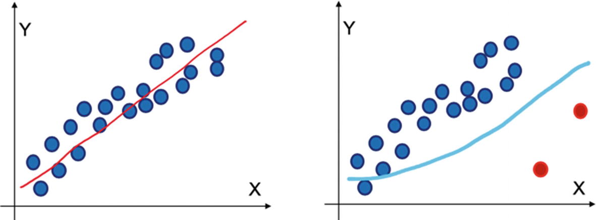 Figure 2-18
Outliers in a dataset seriously impact the accuracy of the regression model since the equation will try to fit the outlier points too; hence, the results will be biased
- b.
Outliers bias the estimates for the model and increase the error variance.
- c.
If a statistical test is to be performed, its power and impact take a serious hit.
- d.
Overall, from the data analysis, we cannot trust coefficients of the model and hence all the insights from the model will be erroneous.
- a.
We will be dealing with how to detect outliers and how to tackle them in Chapter 5.
Linear regression is one of widely used techniques to predict the continuous variables. The usages are vast and many and across multiple domains. It is generally the first few methods we use to model a continuous variable and it acts as a benchmark for the other ML models.
This brings us to the end of our discussion on linear regression models. Next we will discuss a quite popular family of ML models called tree models or tree-based models. Tree-based models can be used for both regression and classification problems. In this chapter we will be studying only the regression problems and in the next chapter we will be working on classification problems.
Tree-Based Methods for Regression
The next type of algorithms used to solve ML problems are tree-based algorithms . Tree-based algorithms are very simple to comprehend and develop. They can be used for both regression and classification problems. A decision tree is a supervised learning algorithm, hence we have a target variable and depending on the problem it will be either a classification or a regression problem.
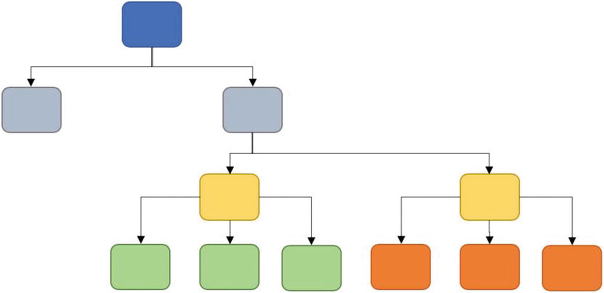
Basic structure of a decision tree shows how iterative decisions are made for splitting
Decision trees can be used to predict both continuous variables and categorical variables. In the case of a regression tree, the value achieved by the terminal node is the mean of the values falling in that region. While in the case of classification trees, it is the mode of the observations. We will be discussing both the methods in this book. In this chapter, we are examining regression problems; in the next chapter classification problems are solved using decision trees.
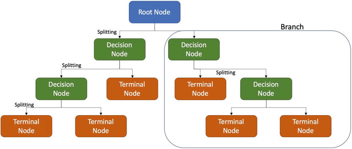
Building blocks of a decision tree consisting of root node, decision node, terminal node, and a branch
- 1.
Root node is the entire population which is being analyzed and is displayed at the top of the decision tree.
- 2.
Decision node represents the subnode which gets further split into subnodes.
- 3.
Terminal node is the final element in a decision tree. Basically when a node cannot split further, it is the end of that path. That node is called terminal node. Sometimes it is also referred to as leaf.
- 4.
Branch is a subsection of a tree. It is sometimes called a subtree.
- 5.
Parent node and child node are the references made to nodes only. A node which is divided is a parent node and the subnodes are called the child nodes.
Let us now understand the decision tree using the house price prediction problem. For the purpose of understanding, let us assume the first criteria of splitting is area. If the area is less than 100 sq km. then the entire population is split in two nodes as shown in Figure 2-21(i). On the right hand, we can see the next criteria is number of bedrooms. If the number of bedrooms is less than four, the predicted price is 100; otherwise, the predicted price is 150. For the left side the criteria for splitting is distance. And this process will continue to predict the price values.
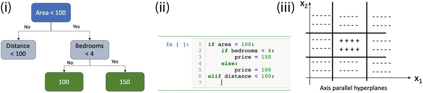
(i) Decision tree based split for the housing prediction problem. (ii) Decision tree can be thought as a nested IF-ELSE block. (iii) Geometric representation of a decision tree shows parallel hyperplanes.
Now you have understood what a decision tree is. Let us also examine the criteria of splitting a node.
A decision tree utilizes a top-down greedy approach . As we know, a decision tree starts with the entire population and then recursively splits the data; hence it is called top-down. It is called a greedy approach, as the algorithm at the time of decision of split takes the decision for the current split only based on the best available criteria, that is, variable and not based on the future splits, which may result in a better model. In other words, for greedy approaches the focus is on the current split only and not the future splits. This splitting takes place recursively unless the tree is fully grown and the stopping criteria is reached. In the case of a classification tree, there are three methods of splitting: Gini index, entropy loss, and classification error. Since they deal with classification problems, we will study these criteria in the next chapter.

We calculate variance for each split as the weighted average of variance for each node. And then the split with a lower variance is selected for the purpose of splitting.
There are quite a few decision tree algorithms available, like ID3, CART, C4.5, CHAID, and so on. These algorithms are explored in more detail in Chapter 3 after we have discussed concepts of classification using a decision tree.
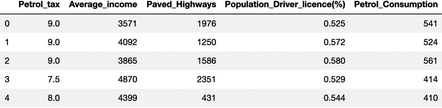
Case study: Petrol consumption using Decision tree
It is time to develop a Python solution using a decision tree. The code and dataset are uploaded to the Github repository. You are advised to download the dataset from the Github link shared at the start of the chapter.
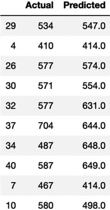
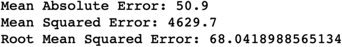
The MAE for our algorithm is 50.9, which is less than 10% of the mean of all the values in the 'Petrol_Consumption' column, indicating that our algorithm is doing a good job.
The visualization of the preceding solution is the code is checked in at GitHub link.

This is the Python implementation of a decision tree. The code can be replicated for any problem we want to solve using a decision tree. We will now explore the pros and cons of decision tree algorithms.
- 1.
Decision trees are easy to build and comprehend. Since they mimic human logic in decision making, the output looks very structured and easy to grasp.
- 2.
They require very less data preparation. They are able to work for both regression and classification problems and can handle huge datasets.
- 3.
Decision trees are not impacted much by collinearity of the variables. The significant variable identification is inbuilt and we validate the outputs of decision trees using statistical tests.
- 4.
Perhaps the most important advantage of decision trees is that they are very intuitive. Stakeholders or decision makers who are not from a data science background can also understand the tree.
- 1.
Overfitting is the biggest problem faced in the decision tree. Overfitting occurs when the model is getting good training accuracy but very low testing accuracy. It means that the model has been able to understand the training data well but is struggling with unseen data. Overfitting is a nuisance and we have to reduce overfitting in our models. We deal with overfitting and how to reduce it in Chapter 5.
- 2.A greedy approach is used to create the decision trees. Hence, it may not result in the best tree or the globally optimum tree. There are methods proposed to reduce the impact of the greedy algorithm like dual information distance (DID). The DID heuristic makes a decision on attribute selection by considering both immediate and future potential effects on the overall solution. The classification tree is constructed by searching for the shortest paths over a graph of partitions. The shortest path identified is defined by the selected features. The DID method considers
- a.
The orthogonality between the selected partitions,
- b.
The reduction of uncertainty on the class partition given the selected attributes.
- a.
- 3.
They are quite “touchy” to the training data changes and hence sometimes a small change in the training data can lead to a change in the final predictions.
- 4.
For classification trees, the splitting is biased towards the variable with the higher number of classes.
We have discussed the concepts of decision tree and developed a case study using Python. It is very easy to comprehend, visualize, and explain. Everyone is able to relate to a decision tree, as it works in the way we make our decisions. We choose the best parameter and direction, and then make a decision on the next step. Quite an intuitive approach!
This brings us towards the end of decision tree–based solutions. So far we have discussed simple linear regression, multinomial regression, nonlinear regression, and decision tree. We understood the concepts, the pros and cons, and the assumptions, and we developed respective solutions using Python. It is a very vital and relevant step towards ML.
But all of these algorithms work individually and one at a time. It allows us to bring forward the next generation of solutions called ensemble methods, which we will examine now.
Ensemble Methods for Regression
“United we stand” is the motto for ensemble methods. They use multiple predictors and then “unite” or collate the information to make a final decision.
Formally put, ensemble methods train multiple predictors on a dataset. These predictor models might or might not be weak predictors themselves individually. They are selected and trained in such a way that each has a slightly different training dataset and may get slightly different results. These individual predictors might learn a different pattern from each other. Then finally, their individual predictions are combined and a final decision is made. Sometimes, this combined group of learners is referred to as meta model.
In ensemble methods, we ensure that each predictor is getting a slightly different data set for training. This is usually achieved at random with replacement or bootstrapping. In a different method, we can adjust the weights assigned to each of the data points. This increases the weights, that is, the focus on those data points.

Ensemble learning–based random forest where raw data is split into randomly selected subfeatures and then individual independent parallel trees are created. The final result is the average of all the predictions by subtrees.
- 1.Bagging models or bootstrap aggregation improves the overall accuracy by the means of several weak models. The following are major attributes for a bagging model:
- a.
Bagging uses sampling with replacement to generate multiple datasets.
- b.
It builds multiple predictors simultaneously and independently of each other.
- c.
To achieve the final decision an average/vote is done. It means if we are trying to build a regression model, the average or median of all the respective predictions will be taken while for the classification model a voting is done.
- d.
Bagging is an effective solution to tackle variance and reduce overfitting.
- e.
Random forest is one of the examples of a bagging method (as shown in Figure 2-22).
- a.
- 2.Boosting : Similar to bagging, boosting also is an ensemble method. The following are the main points about boosting algorithm:
- a.
In boosting, the learners are grown sequentially from the last one.
- b.
Each subsequent learner improves from the last iteration and focuses more on the errors in the last iteration.
- c.
During the process of voting, higher vote is awarded to learners which have performed better.
- d.
Boosting is generally slower than bagging but mostly performs better.
- e.
Gradient boosting, extreme gradient boosting, and AdaBoosting are a few example solutions.
- a.
It is time for us to develop a solution using random forest. We will be exploring more on boosting in Chapter 4, where we study supervised classification algorithms.
Case study: Petrol consumption using Random Forest
For a random forest regression problem, we will be using the same case study we used for decision tree. In the interest of space, we are progressing after creating the training and testing dataset

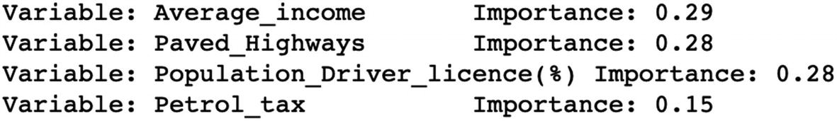
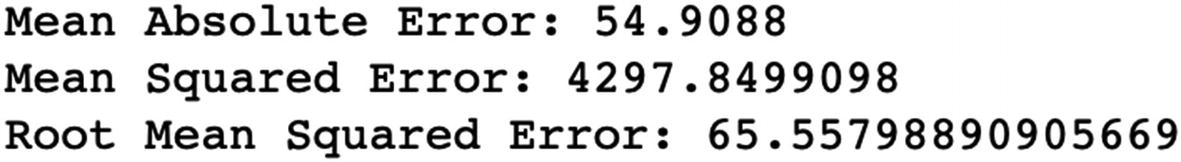
As we can observe, after selecting the significant variables the error has reduced for random forest.
Ensemble learning allows us to collate the power of multiple models and then make a prediction. These models individually are weak but together act as a strong model for prediction. And that is the beauty of ensemble learning. We will now discuss pros and cons of ensemble learning.
- 1.
An ensemble model can result in lower variance and low bias. They generally have a better understanding of the data.
- 2.
The accuracy of ensemble methods is generally higher than regular methods.
- 3.
Random forest model is used to tackle overfitting, which is generally a concern for decision trees. Boosting is used for bias reduction.
- 4.
And most importantly, ensemble methods are a collection of individual models. Hence, more complex understanding of the data is generated.
- 1.
Owing to the complexity of ensemble learning, it is difficult to comprehend. For example, while we can easily visualize a decision tree it is difficult to visualize a random forest model.
- 2.
Complexity of the models does not make them easy to train, test, deploy, and refresh, which is generally not the case with other models.
- 3.
Sometimes, ensemble models take a long time to converge and train. And that increases the training time.
We have covered the concept of ensemble learning and developed a regression solution using random forest. Ensemble learning has been popular for a long time and has won quite a few competitions in Kaggle. You are advised to understand the concepts and replicate the code implementation.
Before we close the discussion on ensemble learning, we have to study an additional concept of feature selection using decision tree. Recall from the last section where we developed a multiple regression problem; we will be continuing with the same problem to select the significant variables.
Feature Selection Using Tree-Based Methods
We are continuing using the dataset we used in the last section where we developed a multiple regression solution using house data. We are using ensemble-based ExtraTreeClassifier to select the most significant features.
The initial steps of importing the libraries and dataset remain the same.

The output shows that the total number of variables was 30; from that list, 11 variables have been found to be significant.
Using ensemble learning–based ExtraTreeClassifier is one of the techniques to shortlist significant variables. We can look at the respective p-values and shortlist the variables.
Ensemble learning is a very powerful method to combine the power of weak predictors and make them strong enough to make better predictions. It offers a fast, easy, and flexible solution which is applicable for both classification and regression problems. Owing to their flexibility sometimes we encounter the problem of overfitting, but bagging solutions like random forest tend to overcome the problem of overfitting. Since ensemble techniques promote diversity in the modeling approach and use a variety of predictors to make the final decision, many times they have outperformed classical algorithms and hence have gained a lot of popularity.
This brings us to the end of ensemble learning methods. We are going to revisit them in Chapter 3 and Chapter 4.
So far, we have covered simple linear regression, multiple linear regression, nonlinear regression, decision tree, and random forest and have developed Python codes for them too. It is time for us to move to the summary of the chapter.
Summary
We are harnessing the power of data in more innovative ways. Be it through reports and dashboards, visualizations, data analysis, or statistical modeling, data is powering the decisions of our businesses and processes. Supervised regression learning is quickly and quietly impacting the decision-making process. We are able to predict the various indicators of our business and take proactive measures for them. The use cases are across pricing, marketing, operations, quality, Customer Relationship Management (CRM), and in fact almost all business functions.
And regression solutions are a family of such powerful solutions. Regression solutions are very profound, divergent, robust, and convenient. Though there are fewer use cases of regression problems as compared to classification problems, they still serve as the foundation of supervised learning models. Regression solutions are quite sensitive to outliers and changes in the values of target variables. The major reason is that the target variable is continuous in nature.
Regression solutions help in modeling the trends and patterns, deciphering the anomalies, and predicting for the unseen future. Business decisions can be more insightful in light of regression solutions. At the same time, we should be cautious and aware that the regression will not cater to unseen events and values which are not trained for. Events such as war, natural calamities, government policy changes, macro/micro economic factors, and so on which are not planned will not be captured in the model. We should be cognizant of the fact that any ML model is dependent on the quality of the data. And for having an access to clean and robust dataset, an effective data-capturing process and mature data engineering is a prerequisite. Then only can the real power of data be harnessed.
In the first chapter, we learned about ML, data and attributes of data quality, and various ML processes. In this second chapter, we have studied regression models in detail. We examined how a model is created, how we can assess the model’s accuracy, pros and cons of the model, and implementation in Python too. In the next chapter, we are going to work on supervised learning classification algorithms.
You should be able to answer the following questions.
Question 1: What are regression and use cases of regression problem?
Question 2: What are the assumptions of linear regression?
Question 3: What are the pros and cons of linear regression?
Question 4: How does a decision tree make a split for a node?
Question 5: How does an ensemble method make a prediction?
Question 6: What is the difference between the bagging and boosting approaches?
Predict the sepal length of the iris flowers using linear regression and decision tree and compare the results.
Question 8: Load the auto-mpg.csv from the Github link and predict the mileage of a car using decision tree and random forest and compare the results. Get the most significant variables and re-create the solution to compare the performance.
Question 9: The next dataset contains information about the used cars listed on www.cardekho.com. It can be used for price prediction. Download the dataset from https://www.kaggle.com/nehalbirla/vehicle-dataset-from-cardekho, perform the EDA, and fit a linear regression model.
Question 10: The next dataset is a record of seven common species of fish. Download the data from https://www.kaggle.com/aungpyaeap/fish-market and estimate the weight of fish using regression techniques.
Question 11: Go through the research papers on decision trees at https://ieeexplore.ieee.org/document/9071392 and https://ieeexplore.ieee.org/document/8969926.
Question 12: Go through the research papers on regression at https://ieeexplore.ieee.org/document/9017166 and https://agupubs.onlinelibrary.wiley.com/doi/full/10.1002/2013WR014203.