
“Prediction is very difficult, especially if it’s about the future.”
— Niels Bohr
We live in a world where the predictions for an event help us modify our plans. If we know that it is going to rain today, we will not go camping. If we know that the share market will crash, we will hold on our investments for some time. If we know that a customer will churn out from our business, we will take some steps to lure them back. All such predictions are really insightful and hold strategic importance for our business.
It will also help if we know the factors which make our sales go up/down or make an email work or result in a product failure. We can work on our shortcomings and continue the positives. The entire customer-targeting strategy can be modified using such knowledge. We can revamp the online interactions or change the product testing: the implementations are many. Such ML models are referred to as classification algorithms, the focus of this chapter.
In Chapter 2, we studied the regression problems which are used to predict a continuous variable. In this third chapter we will examine the concepts to predict a categorical variable. We will study how confident we are for an event to happen or not. We will study logistic regression, decision tree, k-nearest neighbor, naïve Bayes, and random forest in this chapter. All the algorithms will be studied; we will also develop Python code using the actual dataset. We will deal with missing values, duplicates, and outliers, do an EDA, measure the accuracy of the algorithm, and choose the best algorithm. Finally, we will solve a case study to complete the understanding.
Technical Toolkit Required
We are using Python 3.5+ in this book. You are advised to get Python installed on your machine. We are using Jupyter notebook; installing Anaconda-Navigator is required for executing the codes.
The major libraries used are numpy, pandas, matplotlib, seaborn, scikitlearn, and so on. You are advised to install these libraries in your Python environment. All the codes and datasets have been uploaded at the Github repository at the following link: https://github.com/Apress/supervised-learning-w-python/tree/master/Chapter%203
Before starting with classification “machine learning,” it is imperative to examine the statistical concept of critical region and p-value, which we are studying now. They are useful to judge the significance for a variable out of all the independent variables. A very strong and critical concept indeed!
Hypothesis Testing and p-Value
Imagine a new drug X is launched in the market, which claims to cure diabetes in 90% of patients in 5 weeks. The company tested on 100 patients and 90 of them got cured within 5 weeks. How can we ensure that the drug is indeed effective or if the company is making false claims or the sampling technique is biased?
Hypothesis testing is precisely helpful in answering the questions asked.
In hypothesis testing, we decide on a hypothesis first. In the preceding example of a new drug, our hypothesis is that drug X cures diabetes in 90% of patients in 5 weeks. That is called the null hypothesis and is represented by H0. In this case, H0 is 0.9. If the null hypothesis is rejected based on evidence, an alternate hypothesis H1 needs to be accepted. In this case, H1 < 0.9. We always start with assuming that the null hypothesis is true.
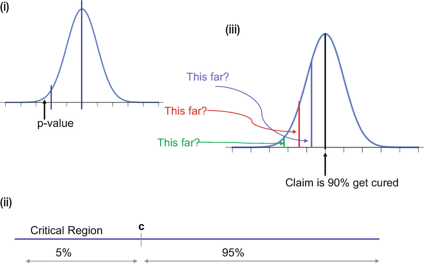
(i) The significance level has to be specified, that is, until what point we will accept the results and not reject the null hypothesis. (ii) The critical region is the 5% region shown in the middle image. (iii) The right side image is showing the p-value and how it falls in the critical region in this case.
We then define the critical region as “c” as shown in Figure 3-1(ii).
If X represents the number of diabetic patients cured, the critical region is defined as P(X<c) < α where α = 5%. In a 95% confidence interval, there is a 5% chance that the sample will not have the population mean. It is interpreted as, if a sample we are interested in falls in a critical region then we can safely reject the null hypothesis.
This is precisely the reason for 5% or 0.05 being referred to as the significance level. If we want a confidence interval of 99%, then 0.01 is the significance level.
Then the next step is to get the p-value. Refer to Figure 3-1(iii) for better understanding.
Formally out, p-value is the probability of getting a value up to and including the one in the sample in the direction of the critical region. It is a method to check if the results of a sample fall in the critical region of the hypothesis test. So, based on the p-value we take a call to reject or accept the null hypothesis.
Once the p-value is calculated, we analyze if the value falls in the critical region. If the answer we get is yes, we can reject the null hypothesis.
This knowledge of hypothesis testing and p-value is critical as it paves the way for identifying the significant variables. Whenever we train our ML algorithms, along with other results we get a p-value for each of the variables. As a rule of thumb, if the p-value is less than or equal to 0.05, the variable is considered as significant.
In this case, the null hypothesis is that the independent variable is not significant and does not impact the target variable. If the p-value is less than or equal to 0.05, we can reject the null hypothesis and hence can conclude that the variable is indeed significant. In the language of statistics, if the p-value for an independent variable x is less than or equal to 0.05, it suggests strong evidence against the null hypothesis as there is less than a 5% chance of the null hypothesis being correct. Or in other words, the variable x is a significant variable to make a prediction for the target variable y. But it does not mean there is 95% probability for the alternate hypothesis to be correct. To be noted is that p-value is a condition upon the null hypothesis and is unrelated to the alternate hypothesis.
We use the p-value to shortlist the significant variables and compare their respective importance. It is a universally accepted metric to choose significant variables.
We will now proceed to the concepts of classification algorithms in the next section.
Classification Algorithms
In our day-to-day business, we make decisions to either invest in stock or not, send a communication to a customer or not, accept a product or reject it, accept an application or ignore it. The basis of these decisions is some sort of insight we have about our business, our processes, our goals, and the factors which enter into our decision making. At the same time, we do expect a favorable output from this decision of ours.
Supervised classified algorithms are used to generate such insights and help us take that decision. They predict the probability for an event to happen or not. At the same time, depending on the choice of supervised learning algorithm, we get to know the factors which impact the occurrences of such an event.
Formally put, classification algorithms are a branch of supervised ML algorithms which are used to model the probability for a certain class. For example, if we want to perform binary classification, we will be modeling for two classes like pass or fail, healthy or sick, fraudulent or genuine, yes or no, and so on. It can be extended to multiclass classification problems—for example, good/bad/neutral, red/yellow/blue/green, cat/dog/horse/car, and so on.
Like a regression model, there is a target variable and independent variables. The only difference is that the target variable is categorical in nature. The independent variables used to make the predictions can be continuous or categorical, and it depends on the algorithm used for modeling.
- 1.
A retailer is losing its repeat customers, that is, customers who used to make purchases are not coming back. The supervised learning algorithm will help identify the customers who are more prone to churn and not come back. The retailer can then target those customers selectively and can offer discounts to bring them back to the business.
- 2.
A manufacturing plant has to maintain the best quality of their products. And for that the technical team would like to ascertain if a particular combination of tools, raw materials, and physical conditions will lead to the best quality and yield. Supervised algorithms can help in that selection.
- 3.
An insurance provider wants to model which customers should be given the policy or not. Depending on the customers’ previous history, employment details, transaction patterns, and so on, the decision has to be made. Here the classification ML model can help to predict acceptance score for the customers, which can be used to accept or reject the application.
- 4.
A bank offering credit cards to its customers has to identify which incoming transactions are fraudulent and which are genuine. Based on the transaction details like origin, amount, time of transaction, mode, and other customer parameters, a decision has to be made. Supervised classification algorithms will be helpful to making that decision.
- 5.
A telecom operator wishes to launch a new data product in the market. For it, the need is to target a few subscribers who have a higher probability of being interested in the product and recharging with it. Supervised classification algorithms will be able to generate a score for each subscriber and subsequently an offer can be made.
The preceding use cases are some of the pragmatic implementations in the industry. A classification algorithm generates a probability score for an event and accordingly the sales/marketing/operations/quality/risk teams can take a business call. Quite a powerful usage and very handy too!
There are quite a few algorithms which serve the purpose and we will be discussing a few in this chapter and rest in Chapter 4.
Logistic regression
k-nearest neighbor
Decision tree
Random forest
Naïve Bayes
SVM
Gradient boosting
Neural networks
We are discussing the first five algorithms in this chapter and rest in the next chapter. Let us start the discussion with the logistic regression algorithm in the next section.
Logistic Regression for Classification
In Chapter 2 we learned how to predict the value for a continuous variable like number of customers, sales, rainfall, and so on using linear regression. Now we have to predict whether a customer will visit or not, whether the sale will go up or not, and so on. Using logistic regression, we can model and solve the preceding problems.
Formally put, logistic regression is a statistical model that utilizes logit function to model classification problems, that is, a categorical dependent variable. In the basic form, we model a binary classification problem and refer to it as binary logistic regression. In complex problems, where more than one categories have to be modeled, we use multinomial logistic regression.
Let us understand logistic regression by means of an example.
Consider we have to make a decision whether a credit card transaction is fraudulent or not. The response is binary (Yes or No); if the transaction seems promising it will be accepted, otherwise not. We will have incoming transaction attributes like amount, time of transaction, payment mode, and so on, and we have to make a decision based on them.
For such a problem, logistic regression models the probability of fraud. In the preceding case, the probability of fraud can be
Probability (fraud = Yes | amount)
The value for this probability will lie between 0 and 1. It can be interpreted as follows: given a value of “fraud amount” we can make a prediction for the genuineness of a credit card transaction.

If we want to predict for “success” using “amount” by fitting the preceding formula, it can be represented in the form of the following graph. For the smaller values of the fraud amount, we can see that probability is less than zero while for the large values, fraud probability is greater than one. And both of these situations are not possible.


(i) Linear regression function will not be able to do justice to the task of predicting fraud. (ii) Logistic regression having an “S”-shaped curve will be more suitable as it will give scores between 0 and 1.

The next question that comes to mind is how to fit this equation. Recall in the case of linear regression, we want to make a prediction of the target variable as close to the actual values. A similar approach is followed here too. The fitting of the logistic regression is done using the maximum likelihood function. The likelihood function measures the goodness of fit of a statistical model and for logistic regression sometimes referred to as log-likelihood function. The mathematical proof is beyond the scope of the book.


In Equation 3-5, the quantity  is referred to as odds. It iscalled odds because it is more intuitive as compared to probability, as odds are a common jargon in betting.
The term log  is called logit. If we compare with a linear regression equation, we can easily make out that with each unit increase in x, the logit (or sometimes called log-odds) changes by β1. This value can take any value between 0 and infinity. We can visualize the function in Figure 3-2(ii).

But there is a question which still remains unanswered: why do we need logistic regression when we have linear regression with us?
If we treat the target variable as a continuous variable, it means we have to predict the actual value of y. But this implies that positive is one less than negative and negative is one less than neutral. And the difference between positive and negative is the same as the difference between negative and neutral. This argument is intrinsically wrong and does not make any practical sense.
Moreover, even if we reduce the number of responses from three to two, let’s say positive and negative only, then too the linear regression might give us some probability score beyond 1 or less than 0, which is mathematically not possible. If we fit the best-found regression line, it still won’t be enough to decide any point by which we can differentiate between the two classes. It will classify some positive as negative and vice versa. Moreover, if we get a score of 0.5 from linear regression, should it be classified as positive or negative? And an outlier can completely mess the outputs for us. Hence it is practically more sensible to use a classification algorithm like logistic regression instead of a linear regression model to solve the problem.
- 1)
Being a classification algorithm, the outcome of the logistic regression model is a binary or dichotomous variable like success/fail, yes/no, or zero/one.
- 2)
There exists a linear relationship between the logit of the outcome and each of the independent variables.
- 3)
Outliers do not exist or at least there are no significant outliers for continuous variables.
- 4)
There exists no correlation between the independent variables.
An important point to be noted is that the accuracy of the algorithm depends on the training data which has been used to train the algorithm. If the training data is not representative, then the resultant model will not be a robust one. The training data should conform to the data quality standards we discussed in Chapter 1. We will be revisiting this concept in detail in Chapter 5.
To be able to have a representative dataset, it is advisable to have a minimum of 10 data points for each of the independent variables with reference to their least frequent value. For example, for 20 independent variables and a least frequent outcome of 0.2, we should have (20*10)/0.2 = 1000 data points.
- 1)
The output of a logistic classification model generally is a probability score for an event. It can be used for both binary classification and multi classification problems.
- 2)
Since the output is probability, it cannot go beyond 1 and cannot be less than 1. And hence the shape of the logistic curve is “S”.
- 3)
It can handle any number of classes as the target variable as well as both categorical and continuous independent variables.
- 4)
The maximum likelihood algorithm helps to determine the respective coefficients for the equation. It is not required for the independent variables to be normally distributed or have an equal variance in each group.
- 5)
 is the odds ratio and whenever this value is positive, the chances of success are above 50%.
 - 6)
The interpretation of coefficients is difficult in logistic regression as the relation is not straightforward as in the case of linear regression.
Before moving further, it is imperative to carefully examine the accuracy measurement methods. You are advised to be thorough with each of them. A vital component in supervised learning, indeed!
Assessing the Accuracy of the Solution
The objective to create an ML solution is to predict for future events. But before deploying the model to a production environment, it is imperative we measure the performance of the model. Moreover, we generally train multiple algorithms with multiple iterations. We have to choose the best algorithm based on the variously accurate KPIs. In this section, we are studying the most important accuracy assessment criteria.
- 1.
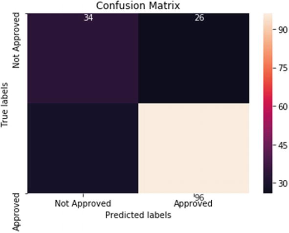
Confusion matrix : One of the most popular methods is confusion matrix. It can be used for both binary and multiclass problems. In its simplest form it is represented as a 2×2 matrix in Figure 3-3.

Confusion matrix is a great way to measure the efficacy of an ML model. Using it, we can calculate precision, recall, accuracy, and F1 score to get the model’s performance.
We will now learn about each of the parameters separately:
- a.
Accuracy: Accuracy is how many predictions were made correctly. In the preceding example, the accuracy is (131+27)/ (131+27+3+24) = 85%
- b.
Precision: Precision represents out of positive predictions; how many were actually positive. In the preceding example, precision is 131/ (131+24) = 84%
- c.
Recall or sensitivity: Recall is how of all the actual positive events; how many we were able to capture. In this example, 131/ (131+3) = 97%
- d.
Specificity or true negative rate: Specificity is out of actual negatives; how many were predicted correctly. In this example: 27/ (27+24) = 92%
- 2.ROC curve and AUC value: ROC or receiver operating characteristics is used to compare different models. It is a plot between TPR (true positive rate) and FPR (false positive rate). The area under the ROC curve (AUC) is a measure of how good a model is. The higher the AUC values, the better the model, as depicted in Figure 3-4. The straight line at the angle of 45° represents 50% accuracy. A good model is having an area above 0.5 and hugging to the top left corner of the graph as shown in Figure 3-4. The one in the green seems to be the best model here.
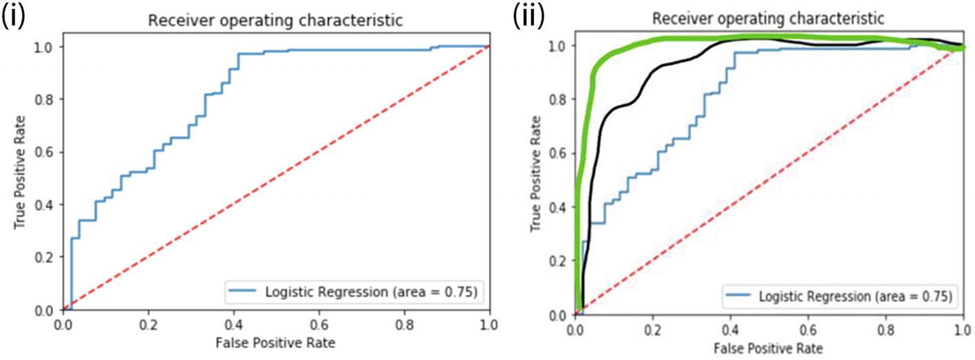 Figure 3-4
(i) ROC curve is shown on the left side. (ii) Different ROC curves are shown on the right. The green ROC curve is the best; it hugs to the top left corner and has the maximum AUC value.
- 3.
Gini coefficient: We also use Gini coefficient to measure the goodness of a fit of our model. Formally put, it is the ratio of areas in a ROC curve and is a scaled version of the AUC.
 (Equation 3-7)
Similar to AUC values, a higher-value Gini coefficient is preferred.
- 4.
F1 score: Many times, we face the problem of which KPI to choose (i.e., higher precision or higher recall) when we are comparing the models. F1 score solves this dilemma for us.
 (Equation 3-8)
F1 score is the harmonic mean of precision and recall. The higher the F1 score, the better.
- 5.
AIC and BIC: Akaike information criteria (AIC) and Bayesian information criteria (BIC) are used to choose the best model. AIC is derived from most frequent probability, while BIC is derived from Bayesian probability.
 (Equation 3-9)while
 (Equation 3-10)
In both formulas, N is number of examples in training set, LL is log-likelihood of the model on training dataset, and k is the number of variables in the model. The log in BIC is natural log to the base e and is called natural algorithm.
We prefer lower values of AIC and BIC. AIC penalizes the model for its complexity, but BIC penalizes the model more than AIC. If we have a choice between the two, AIC will choose a more complex model as compared to BIC.
Given a choice between a very complex model and a simple model with comparable accuracy, choose the simpler one. Remember, nature always prefers simplicity!
- 6.
Concordance and discordance: Concordance is one of the measures to gauge your model. Let us first understand the meaning of concordance and discordance.
Consider if you are building a model to predict if a customer will churn from the business or not. The output is the probability of churn. The data is shown in Table 3-1.Table 3-1Respective Probability Scores for a Customer to Churn or Not
Cust ID
Probability
Churn
1001
1
0.75
2001
0
0.24
3001
1
0.34
4001
0
0.62
Group 1: (churn = 1): Customer 1001 and 3001
Group 2: (churn = 0): Customer 2001 and 4001
Now we create the pairs by taking a single data point from Group 1 and one for Group 2 and then compare them. Hence, they will look like this:
Pair 1: 1001 and 2001
Pair 2: 1001 and 4001
Pair 3: 3001 and 2001
Pair 4: 3001 and 4001
By analyzing the pairs, we can easily make out that in the first three pairs the model is classifying the higher probability as churners. Here the model is correct in the classification. These pairs are called concordant pairs. Pair 4 is where the model is classifying the lower probability as churner, which does not make sense. This pair is called discordant. If the two pairs have comparable probabilities, this is referred to as tied pairs.
We can measure the quality using Somers D, which is given by
Somers D = (percentage concordant pair – percentage discordant pair). The higher the Somers D, the better the model.
Concordance alone cannot be a parameter to make a model selection. It should be used as one of the measures and other measures should also be checked.
- 7.
KS stats: KS statistics or Kolmogorov-Smirnov statistics is one of the measures to gauge the efficacy of the model. It is the maximum difference between the cumulative true positive and cumulative false positive. The higher the KS, the better the model.
- 8.It is also a recommended practice to test the performance of the model on the following datasets and compare the KPIs:
- a.
Training dataset: the dataset used for training the algorithm
- b.
Testing dataset: the dataset used for testing the algorithm
- c.
Validation dataset: this dataset is used only once and in the final validation stage
- d.
Out-of-time validation: It is a good practice to have out-of-time testing. For example, if the training/testing/validation datasets are from Jan 2015 to Dec 2017, we can use Jan 2018–Dec 2018 as the out-of-time sample. The objective is to test a model’s performance on an unseen dataset.
- a.
These are the various measures which are used to check the model’s accuracy. We generally create more than one model using multiple algorithms. And for each algorithm, there are multiple iterations done. Hence, these measures are also used to compare the models and pick and choose the best one.
There is one more point we should be cognizant of. We would always want our systems to be accurate. We want to predict better if the share prices are going to increase or decrease or whether it will rain tomorrow or not. But sometimes, accuracy can be dubious. We will understand it with an example.
For example, while developing a credit card fraud transaction system our business goal is to detect transactions which are fraudulent. Now generally most (more than 99%) of the transactions are not fraudulent. This means that if a model predicts each incoming transaction as genuine, still the model will be 99% accurate! But the model is not meeting its business objective of spotting fraud transactions. In such a business case, recall is the important parameter we should target.
With this, we conclude our discussion of accuracy assessment. Generally, for a classification problem, logistic regression is the very first algorithm we use to baseline. Let us now solve an example of a logistic regression problem.
Case Study: Credit Risk
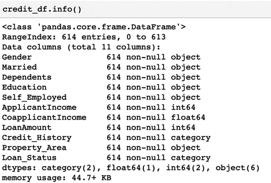
Business Context: Credit risk is nothing but the default in payment of any loan by the borrower. In the banking sector, this is an important factor to be considered before approving the loan of an applicant. Dream Housing Finance company deals in all home loans. They have presence across all urban, semiurban, and rural areas. Customers first apply for a home loan; after that company validates the customers’ eligibility for the loan.
Business Objective : The company wants to automate the loan eligibility process (real time) based on customer detail provided while filling out the online application form. These details are gender, marital status, education, number of dependents, income, loan amount, credit history, and others. To automate this process, they have given a problem to identify the customer segments that are eligible for loan amounts so that they can specifically target these customers. Here they have provided a partial dataset.
Dataset: The dataset and the code is available at the Github link for the book shared at the start of the chapter. A description of the variables is given in the following:
- a.
Loan_ID: Unique Loan ID
- b.
Gender: Male/Female
- c.
Married: Applicant married (Y/N)
- d.
Dependents: Number of dependents
- e.
Education: Applicant Education (Graduate/Undergraduate)
- f.
Self_Employed: Self-employed (Y/N)
- g.
ApplicantIncome: Applicant income
- h.
CoapplicantIncome: Coapplicant income
- i.
LoanAmount: Loan amount in thousands
- j.
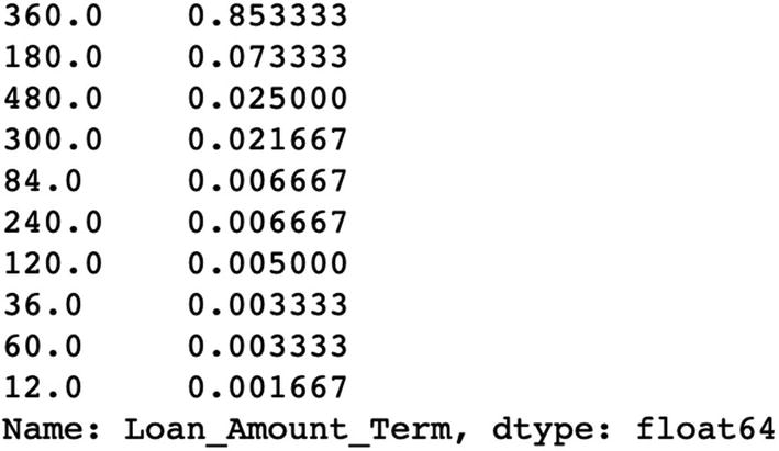
Loan_Amount_Term: Term of loan in months
- k.
Credit_History: credit history meets guidelines
- l.
Property_Area: Urban/ Semi Urban/ Rural
- m.
Loan_Status: Loan approved (Y/N)
Let’s start the coding part using logistic regression. We will explore the dataset, clean and transform it, fit a model, and then measure the accuracy of the solution.


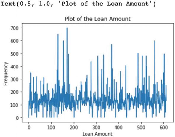
We have shown only one visualization. You are advised to generate more graphs and plots. Remember, plots are a fantastic way to represent data intuitively!

You are advised to create box-plot diagrams as we have discussed in Chapter 2.
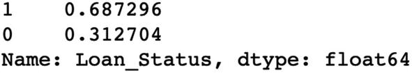
There seems to be a slight imbalance in the dataset as one class is 31.28% and the other is 68.72%.
While the dataset is not heavily imbalanced, we will also examine how to deal with data imbalance in Chapter 5.
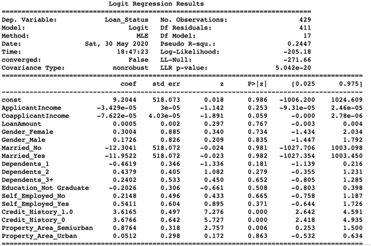
Let us interpret the results. The pseudo r-square shows that only 24% of the entire variation in the data is explained by the model. It is really not a good model!
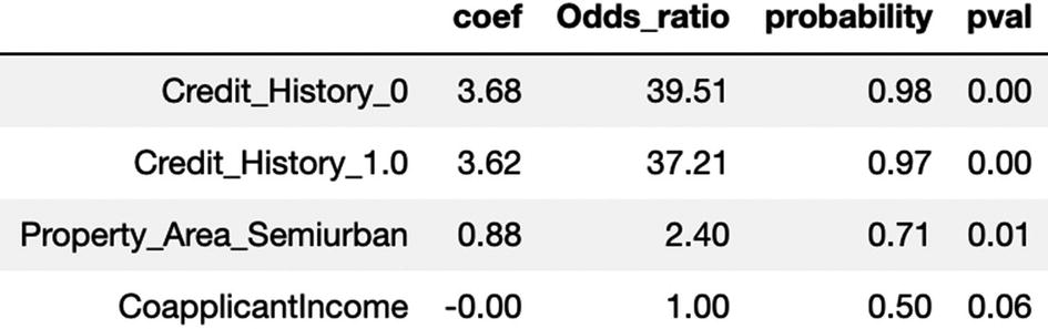
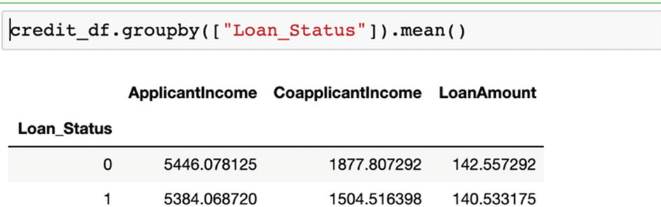
If we analyze the data, we can see that the customers who have credit history 1 have a 97% probability of defaulting the loan while the ones having history of 0 have 98% probability of defaulting.
Similarly, the customers in semiurban areas have odds of 2.50 times to default as compared to others.
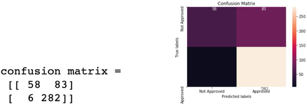
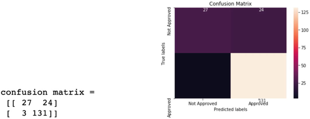


On testing data, the model’s overall accuracy is 85%. Sensitivity or recall is 97% and precision is 84%. The model has a good overall accuracy. However, the model can be improved as we can see that 24 applications were predicted as approved while they were actually not approved.
Additional Notes

If the testing accuracy is not similar to training accuracy and is significantly lower, it means the model is overfitting. We will study how to tackle this problem in Chapter 5.
Logistic regression is generally the first few algorithms which are used whenever we approach a classification problem. It is fast, easy to comprehend, and compact to handle categorical and continuous data points alike. Hence, it is quite popular. It can also be used to get the significant variables for a problem.
Now that we have examined logistic regression in detail, let us move to the second very important classifier used: naïve Bayes. Don’t go by the word “naïve”; this algorithm is quite robust in making classifications!
Naïve Bayes for Classification
Factors to Consider When Planning a Camping Trip
Day off | Weather | Friends coming | Humidity | Going camping |
|---|---|---|---|---|
Yes | Rainy | No | High | Yes |
No | Sunny | Yes | Low | Yes |
Yes | Overcast | No | Low | No |
Yes | Rainy | No | High | Yes |
Yes | Sunny | Yes | Low | Yes |
Yes | Rainy | Yes | High | Yes |
No | Sunny | No | High | No |
No | Overcast | Yes | Low | Yes |
- 1)
If A is any event, then the complement of A, denoted by Â, is the event that A does not occur.
- 2)
The probability of A is represented by P(A), and the probability of its complement P(
 ) = 1 – P(A).
 - 3)
Let A and B be any events with probabilities P(A) and P(B). If you are told that when B has occurred, then the probability of A might change. As in the previous case if the weather is rainy then the probability of camping changes. This new probability of A is called the conditional probability of A given B, which can be written as P(A|B).
- 4)
Mathematically,
 where P(A|B) means that probability of A given B which means the probability of A if B was known to have occurred.
 - 5)
This relationship can be viewed as probabilistic dependency and is called conditional probability. It means that knowledge of one event is of importance when assessing the probability of the other.
- 6)
If the two events are mutually independent, then the multiplication rule simplifies to P (A and B) = P(A)P(B). For example, there will be no impact on your camping plans based on the price of milk.
There are many events which are mutually dependent on each other and hence it becomes imperative to understand the relationship: P(A|B) and P(B|A). This is true in the case of business activities too where the sales are dependent on the number of customers visiting the store, a customer will come back for shopping or not will depend on the previous experiences, and so on. Bayes’ theorem helps to model for such factors and make a prediction.

where P(A) and P(B): probability of A and B respectively, P(A|B): probability of A given B and P(B|A): probability of B given A.
For example, if we want to know in finding out a patient’s probability to have a heart disease if they have diabetes. The data we have is as follows: 10% of patients entering the clinic have heart disease while 5% of the patients have diabetes. Among the patients diagnosed with heart disease, 8% are diabetic. Then P(A) = 0.10, P(B) = 0.05, and P(B|A) = 0.08. And using Bayes’ rule, P(A|B) = (0.08×0.1)/0.05 = 0.16.
If we generalize the rule, let A1 through An be a set of mutually exclusive outcomes. The probabilities of the events A are P(A1) through P(An). These are called prior probabilities. Because an information outcome might influence our thinking about the probabilities of any Ai, we need to find the conditional probability P(Ai|B) for each outcome Ai. This is called the posterior probability of Ai.


Bayes’ theorem is used for making classification (binary or multiclass), and it is referred to as naïve Bayes. It is called naïve due to a very strong assumption that the variables and features are independent of each other which is generally not true in the real world. Often this assumption is violated and still naïve Bayes tends to perform well. The idea is to factor all available evidence in the form of predictors into the naïve Bayes rule to obtain more accurate probability for class prediction.
As per Bayes’ rule, the naïve Bayes estimates conditional probability (i.e., the probability that something will happen, given that something else has already occurred). For example, if we want to design an email spam filter and find a given mail is spam if there is an appearance of the word “discount.” It is easy to implement, fast, robust, and quite accurate. Because of its ease of use, it is quite a popular technique.
- 1.
It is a simple, easy, fast, and very robust method.
- 2.
It does well with both clean and noisy data.
- 3.
It requires few examples for training, but the underlying assumption is that the training dataset is a true representative of the population.
- 4.
It is easy to get the probability for a prediction.
- 1.
It relies on a very big assumption that independent variables are not related.
- 2.
It is generally not suitable for datasets with large numbers of numerical attributes.
- 3.
The predicted probabilities by the naïve Bayes algorithm is considered as less reliable in practice than predicted classes.
- 4.
In some cases, it has been observed that if a rare event is not in training data but present in the test, then the estimated probability will be wrong.
But when some of our independent variables are continuous, we cannot calculate conditional probabilities! And hence in real-life variables, naïve Bayes is extended to Gaussian naïve Bayes.
In Gaussian naïve Bayes, continuous values associated with each attribute or independent variable are assumed to be following a Gaussian distribution. They are also easier to work with, as for the training we would only have to estimate the mean and standard deviation of the continuous variable.
Let us move to the case study to develop the naïve Bayes solution.
Case Study: Income Prediction on Census Data
Business Objective: We have census data and the objective is to predict whether income exceeds 50K/yr for an individual based on the value of other attributes.
Dataset: The dataset and code is available at the Github link shared at the start of this chapter.
Age: continuous
Workclass: Private, Self-emp-not-inc, Self-emp-inc, Federal-gov, Local-gov, State-gov, Without-pay, Never-worked.
fnlwgt: continuous.
Education: Bachelors, Some-college, 11th, HS-grad, Prof-school, Assoc-acdm, Assoc-voc, 9th, 7th-8th, 12th, Masters, 1st-4th, 10th, Doctorate, 5th-6th, Preschool.
Education-num: continuous.
Marital-status: Married-civ-spouse, Divorced, Never-married, Separated, Widowed, Married-spouse-absent, Married-AF-spouse.
Occupation: Tech-support, Craft-repair, Other-service, Sales, Exec-managerial, Prof-specialty, Handlers-cleaners, Machine-op-inspct, Adm-clerical, Farming-fishing, Transport-moving, Priv-house-serv, Protective-serv, Armed-Forces.
Relationship: Wife, Own-child, Husband, Not-in-family, Other-relative, Unmarried.
Race: White, Asian-Pac-Islander, Amer-Indian-Eskimo, Other, Black.
Sex: Female, Male.
Capital-gain: continuous.
Capital-loss: continuous.
Hours-per-week: continuous.
Native-country: United States, Cambodia, England, Puerto Rico, Canada, Germany, Outlying-US (Guam-USVI-etc), India, Japan, Greece, South, China, Cuba, Iran, Honduras, Philippines, Italy, Poland, Jamaica, Vietnam, Mexico, Portugal, Ireland, France, Dominican Republic, Laos, Ecuador, Taiwan, Haiti, Colombia, Hungary, Guatemala, Nicaragua, Scotland, Thailand, Yugoslavia, El Salvador, Trinadad&Tobago, Peru, Hong, Holland-Netherlands.
Class: >50K, <=50K
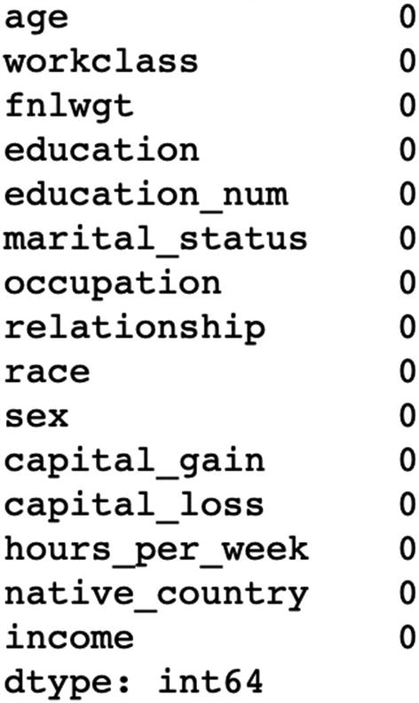
The preceding output shows that there is no “null” value in our dataset.

The output of the preceding code snippet shows that there are 1836 missing values in the workclass attribute, 1843 missing values in the occupation attribute, and 583 values in the native_country attribute.


With it we have implemented naïve Bayes using a live dataset. You are advised to understand each of the steps and practice the solution by replicating it.
Naïve Bayes is a fantastic algorithm to practice and use. Bayesian statistics is gathering a lot of attention and its power is being harnessed in research areas a lot. You might have heard the term Bayesian optimization . The beauty of the Bayes’ theorem lies in its simplicity, which is very much visible in our day-to-day life. A straightforward method indeed!
We have covered logistic regression and naïve Bayes so far. Now we will examine one more very widely used classifier called k-nearest neighbor. One of the popular methods, easy to understand and implement—let’s study knn next.
k-Nearest Neighbors for Classification
“Birds of the same feather flock together .” This old adage is perfect for k-nearest neighbors. It is one of the most popular ML techniques where the learning is based on the similarity of data points with each other. knn is a nonparametric model; it does not construct a “model” and the classification is based on a simple majority vote from the neighbors. It can be used for classification where the relationship between attributes and target classes is complex and difficult to understand, and yet items in a class tend to be fairly homogenous on the values of attributes. But it might not be the best choice for an unclean dataset or where the target classes are not distinctively clear. If the target classes are not clearly demarcated, then it leads to an obvious confusion while taking the majority vote. knn can also be used for regression problems to make a prediction for a continuous variable. In the case of regression, the final output will be the average of the values of the neighbors and that average will be assigned to the target variable. Let us examine this visually:
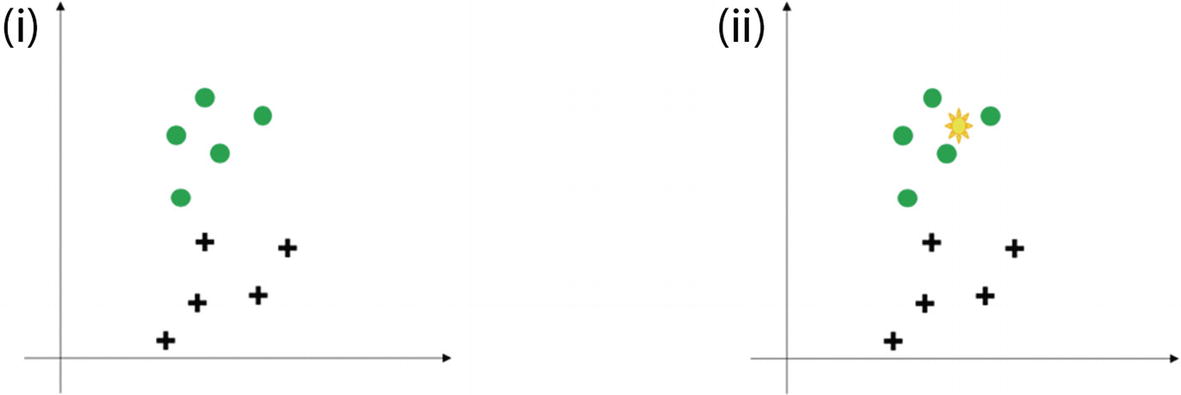
(i) The distribution of two classes in green circle and black plus sign. (ii) The right side shows the new data point which has to be classified (shown in yellow sign). The k-nearest neighbor algorithm has to be used to make the classification.
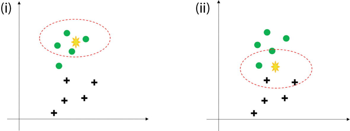
(i) The presence of new unseen data if we select four nearest neighbors. It is an easy decision to make. (ii) The right side shows that the new data point is difficult to classify as the four neighbors are mixed.
The four closest points to the yellow point all belong to circles or we can say that all the neighbors of the unknown yellow point are circles. Hence, with a good confidence level we can predict that the yellow point should belong to the circle. Here the choice was comparatively easy and straightforward. Refer to Figure 3-6(ii), where it is not that simple. Hence, the choice of k plays a very crucial role.
- 1.
We receive the raw and unclassified dataset which has to be worked upon.
- 2.
We choose a distance matrix from Euclidean, Manhattan or Minkowski.
- 3.
Then calculate the distance between the new data points and the known classified training data points.
- 4.
The number of neighbors to be considered is defined by the value of “k”.
- 5.
It is followed by comparing with the list of classes which have the shortest distance and count the number of times each class appears.
- 6.
The class with the highest votes wins. This means that the class which has the highest frequency and has appeared the greatest number of times is assigned to the unknown data point.
Parametric models make some assumptions about the input data like having a normal distribution. However, nonparametric methodology believes that data distributions are undefinable by a finite set of parameters and hence do not make any assumptions.
From the steps discussed for k-nearest neighbor, we can clearly understand that the final accuracy depends on the distance matrix used and the value of “k”.
- 1.
Euclidean Distance : probably the most common and easiest way to calculate between two points. It is square root of the sum of the squares of distances:
 (Equation 3-14)
 - 2.
Manhattan Distance : The distance between two points measured along axes at right angles. Sometimes it is also referred to as city block distance. In a plane with p1 at (x1, y1) and p2 at (x2, y2), it is
 (Equation 3-15)
 - 3.
Minkowski Distance : This is a metric in a normed vector space. Minkowski distance is used for distance similarity of vectors. Given two or more vectors, find the distance similarity of these vectors. Mainly, the Minkowski distance is applied in ML to find out the distance similarity. It is a generalized distance metric and can be represented by the following formula:
 (Equation 3-16)
where by using different values of p we can get different values of distances. With the value of p = 1 we get Manhattan distance, with p = 2 we get Euclidean distance, and with p= ∞ we get Chebychev distance.
- 4.
Cosine Similarity: It is a measure of similarity between two nonzero vectors of an inner product space that measures the cosine of the angle between them. The cosine of 0° is 1, and it is less than 1 for any angle in the interval (0,π] radians.
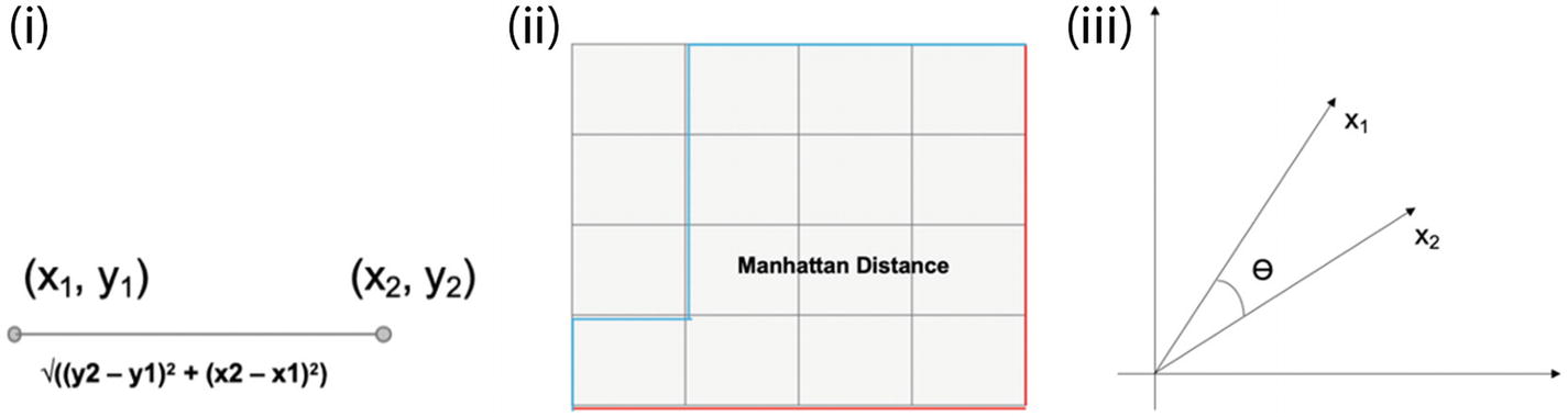
(i) Euclidean distance; (ii) Manhattan distance; (iii) cosine similarity
While approaching a knn problem, generally we start with Euclidean distance. In most business problems, it serves the purpose. Distance matrix is an important parameter in unsupervised clustering methods like k-means clustering.
- 1.
It is a nonparametric method and does not make any assumptions about distributions of the various classes in vector space.
- 2.
It can be used for the binary classification as well as multiclassification problems.
- 3.
The method is quite easy to comprehend and implement.
- 4.
The method is robust and if the value of k is large, it is not impacted by outliers.
- 1.
The accuracy depends on the value of k and hence finding the most optimal value can be a difficulty sometimes.
- 2.
The method requires the class distributions to be non-overlapping.
- 3.
There is no specific output as a model and if the value of k is small, it is negatively impacted by the presence of outliers.
- 4.
The method is calculation intensive as it is a lazy learner. The distances have to be calculated between all the points and then a majority is to be taken. And hence, it is not that fast of a method to use.
There are other forms of knn too, which are as follows:
- 1.
This classifier implements the learning based on a number of neighbors. The neighbors are within a fixed radius r of each training point, where r is a floating point value specified by the user.
- 2.
We prefer this method when the data sampling is not uniform. But, in case of quite a few independent variables and a sparse dataset, it suffers with the curse of dimensionality.
When the number of dimensions increases, the volume of space increases at a very fast pace and the resultant data becomes very sparse. This is called the curse of dimensionality. Data sparsity makes statistical analysis for any dataset quite a challenging task.
- 1.
This method is effective if the dataset is large but the number of independent variables is less.
- 2.
The method takes less time to compute as compared to other methods.
It is now time to create a Python solution using knn, which we are executing next.
Case Study: k-Nearest Neighbor
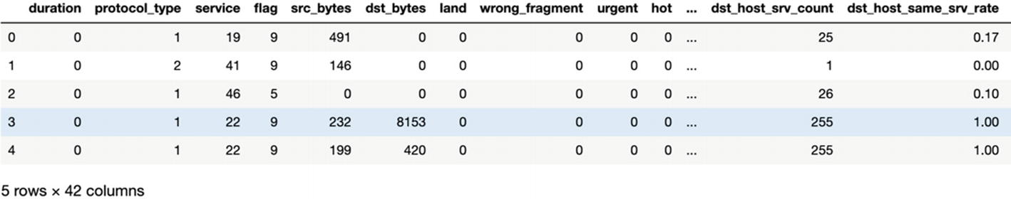
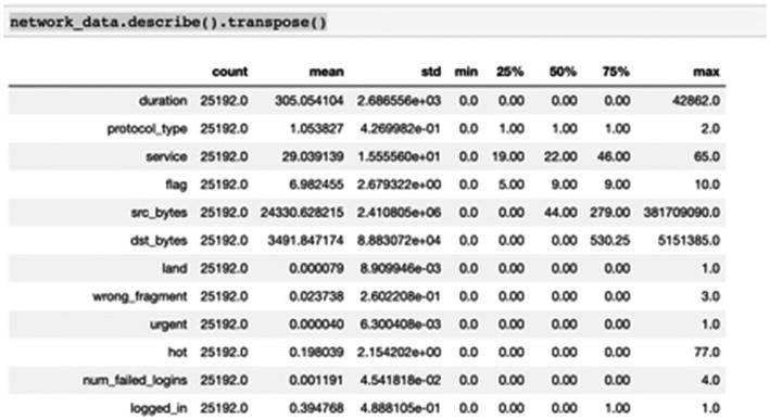
The dataset to be audited, which consists of a wide variety of intrusions simulated in a military network environment, was provided. It created an environment to acquire raw TCP/IP dump data for a network by simulating a typical US Air Force LAN. The LAN was focused like a real environment and blasted with multiple attacks. A connection is a sequence of TCP packets starting and ending at some time duration between which data flows to and from a source IP address to a target IP address under some well-defined protocol. Also, each connection is labeled either as normal or as an attack with exactly one specific attack type. Each connection record consists of about 100 bytes. For each TCP/IP connection, 41 quantitative and qualitative features are obtained from normal and attack data (3 qualitative and 38 quantitative features).
The class variable has two categories: normal and anomalous.
The Dataset
The dataset is available at the git repository as Network_Intrusion.csv file. The code is also available at the Github link shared at the start of the chapter.
Business Objective
We have to fit a k-nearest neighbor algorithm to detect network intrusion.

This dataset does not have any null values; we will study in detail on how to deal with null values, NA, NaN, and so on in Chapter 5.


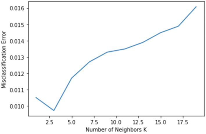
The accuracy and recall are 0.9902758483826156 and 0.9911944869831547 respectively.
With k = 3, we are getting a very good accuracy and a great recall value too. This model can be considered as the final one to be used.
We developed a solution using knn and are getting good accuracies. k-nearest neighbor is very easy to explain and visualize. Not being very statistics- or mathematics-heavy, even for non–data science users, the method is not very tedious to understand. And this is one of the most important properties of this method. Being a nonparametric method, there is no assumption about the data and hence it requires less data preparation.
We have covered logistic regression, naïve Bayes, and k-nearest neighbor. Generally, when we start any classification solution, we start with these three algorithms to check their accuracy. The next in the series are tree-based algorithms: decision tree and random forest. We have discussed the theoretical concepts about both in Chapter 2. In the next section, we will cover the differences and then implement them on a dataset.
Tree-Based Algorithms for Classification

A decision tree is comprised of root node, decision node, and a terminal node. A subtree is called a branch
The difference is the process of splitting followed by a classification algorithm which is discussed now.
Transportation Mode Dependency on Other Factors Like Gender and Income Level
Vehicle Count | Gender | Cost | Income | Transportation Mode |
|---|---|---|---|---|
1 | Female | Less | Middle class | Train |
0 | Male | Less | Low income | Bus |
1 | Female | High | Middle class | Train |
1 | Male | Less | Middle class | Bus |
0 | Male | Medium | Middle class | Train |
1 | Male | Less | Middle class | Bus |
2 | Female | High | High class | Car |
0 | Female | Less | Low income | Bus |
2 | Male | High | Middle class | Car |
1 | Female | High | High class | Car |
Entropy: Entropy and information gain walk hand-in-hand. A pure node will require less information to describe itself while an impure node will require more information. It can be understood in the form of entropy too. (Information gain = 1 – Entropy.)

where p and q are the probability of success and failure, respectively, in that node. The logarithm is to the base of 2 here.
In the preceding example, entropy = –0.4 (log 0.4) – 0.3(log 0.3) – 0.3(log 0.3) = 1.571
Entropy of a pure node is 0 and can be represented as Figure 3-9.

Values of maximum entropy for different numbers of classes (n). Probability p = 1/n.
Gini coefficient : Gini index can also be used to measure the impurity. The formula to be used is as follows:
 (Equation 3-18)
In the preceding example, Gini index = 1 – (0.4^2 + 0.3^2 + 0.3^2) = 0.660
Gini of a node containing a single class is 0 because the probability is 1. Like entropy, it also takes maximum value when all the classes in the node have the same probability. The movement of Gini can be represented as in Figure 3-10.
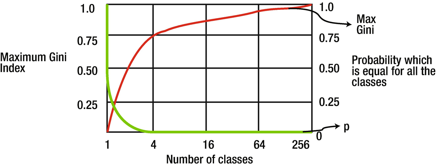
Values of maximum Gini index for different number of classes (n). Probability p = 1/n.
The value of Gini will always be between 0 and 1 irrespective of the number of classes in the model.
Classification Error : The next way to measure the degree of impurity is using classification error. It is given by the formula

where i is the number of classes
Similar to the other two, its value lies between 0 and 1.
For the preceding example, classification error index = 1 – max(0.4,0.3,0.3) = 0.6
We can use any of these three splitting methods for classification. There are some common decision tree algorithms which are used for regression and classification problems. Since we have studied both regression and classification concepts, it is a good time to examine different types of decision tree algorithms, which is the next section.
Types of Decision Tree Algorithms
There are some significant decision tree algorithms which are used in the industry. Some of them are suitable for classification problems while some are a better choice for regression solutions. We are discussing all the aspects of the algorithms.
- 1.
ID3 or Iterative Dichotomizer 3 is a decision tree algorithm using greedy search to split the dataset in each iteration. It uses entropy or information gain as a factor to perform the split iteratively. For each successive iteration in the model, it uses unused variables in the last iteration, calculates the entropy for those unused variables, and then selects the variable with lowest entropy. Or in other words, it selects the variable with highest information gain. ID3 can lead to overfitting and may not be the most optimal choice. It fares quite well with categorical variables. But when the dataset contains continuous variables, it becomes slower to converge since there are many values on which the node splitting can be done.
- 2.
CART or classification and regression tree is a flexible tree-based solution. It can model for both continuous or categorical target variables and hence it is one of the highly used tree-based algorithms. Like a regular decision tree algorithm, we choose input variables and split the nodes iteratively till we achieve a robust tree to work upon. The selection of the input variables is done using a greedy approach with the objective to minimize the loss. The tree construction stops based on a predefined criteria like minimum observations to be present in each of the leaves. Python library scikit-learn uses an optimized version of CART but does not support categorical variables as of now.
- 3.
C4.5 is an extension of ID3 and is used for classification problems. Similar to ID3, it utilizes entropy or information gain to make the split. It is a robust choice since it can handle both categorical and continuous variables. For continuous variables, it assigns a threshold value and does the split based on the threshold. Variables with value above the threshold are in one bucket while variables with threshold less than or equal to threshold are in a different bucket. It allows missing variables in the data as the missing values are not considered while calculating the entropy values.
- 4.
CHAID (Chi-square automatic interaction detection ) is a popular algorithm in the field of market research and marketing; for example, if we want to understand how a certain group of customers will respond to a new marketing campaign. This marketing campaign can be for a new product or service and will be useful for the marketing team to strategize accordingly. CHAID is primarily based on adjusted significance testing and is mostly used when we have a categorical target variable and categorical independent variables. It proves to be quite a handy and convenient method to visualize such a dataset.
- 5.
MARS or multivariate adaptive regression splines is a nonparametric regression technique. It is mostly suitable for measuring nonlinear relationships between variables. It is a flexible regression model which can handle both categorical and continuous variables. It is quite a robust solution to handle massive datasets and requires very much less data preparation, making is comparatively faster to implement. Owing to its flexibility and ability to model nonlinearities in the dataset, MARS generally is a good choice to tackle overfitting in the model.
The tree-based algorithms discussed previously are unique in their own way. Some of them are more suitable for classification problems, while some are a better choice for regression problems. CART can be used for both classification and regression problems.
Now it is time to develop a case study using decision tree.
The code and the dataset are available at the Github link shared at the start of this chapter.
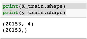
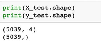
We can use the same dataset we have used for the logistic regression problem. The implementation follows after we have created the training and testing data.
We will now model the same problem using a random forest model. Recall that random forest is an ensemble-based technique where it creates multiple smaller trees using a subset of data. The final decision is based on the voting mechanism by each of the trees. In the last chapter, we have used random forest for a regression problem; here we are using random forest for a classification problem.
Decision trees are generally prone to overfitting; ensemble-based random forest model is a good choice to tackle overfitting.
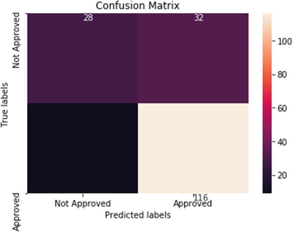
This is the implementation of a decision tree algorithm and ensemble-based random forest algorithm. Tree-based algorithms are very easy to comprehend and implement. They are generally the first few algorithms which we implement and test the accuracy of the system. Tree-based solutions are recommended if we want to create a quick solution, but they are prone to overfitting. We can use tree pruning or setting a constraint on tree size to overcome overfitting. We will again visit this concept in Chapter 5, in which we will discuss all the techniques to overcome the problem of overfitting in our ML model.
With this, we come to the end of our discussion on tree-based algorithms. In this chapter, we have studied the classification algorithms and implemented them too. These algorithms are quite popular in the industry and powerful enough to help us make a robust ML model. Generally, we test the data on these algorithms at the start and then choose the one which is giving us the best results. And then we tune it further till we achieve the most desirable output. The desirable output may not be the most complex solution but surely will be one which will deliver the desired level of measurement parameters, reproducibility, robustness, flexibility, and ease of deployment. Remember, complexity is not proportional to accuracy. A more complex model does not mean a higher degree of performance!
Summary
Prediction is a powerful tool in our hands. Using these ML algorithms, we can not only take a confident decision we can also ascertain the factors which affect that decision. These algorithms are heavily used across sectors like banking, retail, manufacturing, insurance, aviation, and so on. The uses include fraud detection, quality inspection, churn prediction, loan default prediction, and so on.
You should note that these algorithms are not the only sources of knowledge. A sound exploratory analysis is a prerequisite for a good ML algorithm. And the most important resource is “data” itself. A good-quality and representative dataset is of paramount importance. We have discussed the qualities of a good dataset in Chapter 1.
It is also imperative that a sound business problem has been created from the start. The choice of the target variable should align with the business problem at hand. The training data used to train the algorithm plays a very crucial role, as on it depends the patterns learned by the algorithm. It is important to note that we do measure the performance of the algorithms using the various parameters like precision, recall, AUC, F1 score, and so on. An algorithm which is performing well on training, testing, and validation datasets will be the best algorithm. But still there are a few other parameters based on which we choose the final algorithm which can be deployed into production, which we discuss in Chapter 5.
In Chapter 1, we examined ML, various types, data and attributes of data quality and ML process. In Chapter 2, we studied ML algorithms to model a continuous variable. In this third chapter, we complemented the knowledge with classification algorithms. These first chapters have created a firm base for you to solve most of the business problems in the data science world. Also, you are now ready to take the next step in Chapter 4.
In the first three chapters, we have discussed basic and intermediate algorithms. In the next chapter, we are going to cover much more complex algorithms like SVM, gradient boosting, and neural networks for regression and classification problems. So stay focused!
Question 1: How does a logistic regression algorithm make a classification prediction?
Question 2: What is the difference between precision and recall?
Question 3: What is posterior probability?
Question 4: What are the assumptions in a naïve Bayes algorithm?
Question 5: How can we choose the value of k in k-nearest neighbor?
Question 6: What are the various performance measurement parameters for classification algorithms?
Question 7: The sinking of the ship Titanic in 1912 was indeed heart-breaking. Some passengers survived, some did not. Download the dataset from https://www.kaggle.com/c/titanic. Using ML, predict which passengers were more likely to survive than others based on the various attributes of the passengers.
We have worked upon the same dataset in the last chapter. Here, you have to classify the type of the flower using classification algorithms and compare the results.
Question 9: Download the Bank Marketing Dataset from the link https://archive.ics.uci.edu/ml/datasets/Bank+Marketing. The data is related with direct marketing campaigns (phone calls) of a Portuguese banking institution. The classification problem goal is to predict if the client will subscribe to a term deposit. Create various classification models and compare the respective KPIs.
Question 10: Get the German Credit Risk data from https://www.kaggle.com/uciml/german-credit. The dataset contains attributes of each person who takes credit from the bank. The objective is to classify each person as a good or bad credit risk according to their attributes. Use classification algorithms to create the model and choose the best model.
Question 11: Go through the research paper on logistic regression at https://www.ncbi.nlm.nih.gov/pmc/articles/PMC6696525/.
Question 12: Go through the research paper on random forest at https://aip.scitation.org/doi/pdf/10.1063/1.4977376. There is one more good paper at https://aip.scitation.org/doi/10.1063/1.4952607.
Question 13: Examine the research paper on knn at https://pdfs.semanticscholar.org/a196/39771e987588b378879c65300b61b4af86af.pdf.
Question 14: Study the research paper on naïve Bayes at https://www.cc.gatech.edu/~isbell/reading/papers/Rish.pdf.