
Chapter Nineteen. Landform Drawings
Objectives
After studying the material in this chapter, you should be able to:
1. Read and draw a plat, topographic contour map, street contour map, and highway plan and profile.
2. Read the elevation of a tract of land using contour lines.
3. Identify the scale and compass orientation of a topographic map.
4. Read and notate property boundaries on a land survey map.
5. Create a profile map from contour lines.
Understanding Landform Drawings
The purpose of a landform drawing or map determines the features and details to show on it and the scale to use. Many types of maps and drawings are used to locate features on the Earth’s surface.
Because the shape of the Earth is spherical, any representation on a plane (such as a piece of paper) is distorted because spheres can be developed into a flat plane only by approximation. When drawing large areas, you can define control or reference points using spherical coordinates for latitude and longitude (meridians and parallels) as reference lines to minimize the distortion. In drawing small areas to a relatively large scale, the distortion due to the Earth’s curvature is so slight that it may be neglected.
Definitions
Useful map and landform drawing terms include the following.
A plat is a map of a small area, plotted from a land survey. It does not ordinarily show elevations. Plats are drawn to calculate areas, locate property lines, and locate building projects and facilities (Figure 19.1).
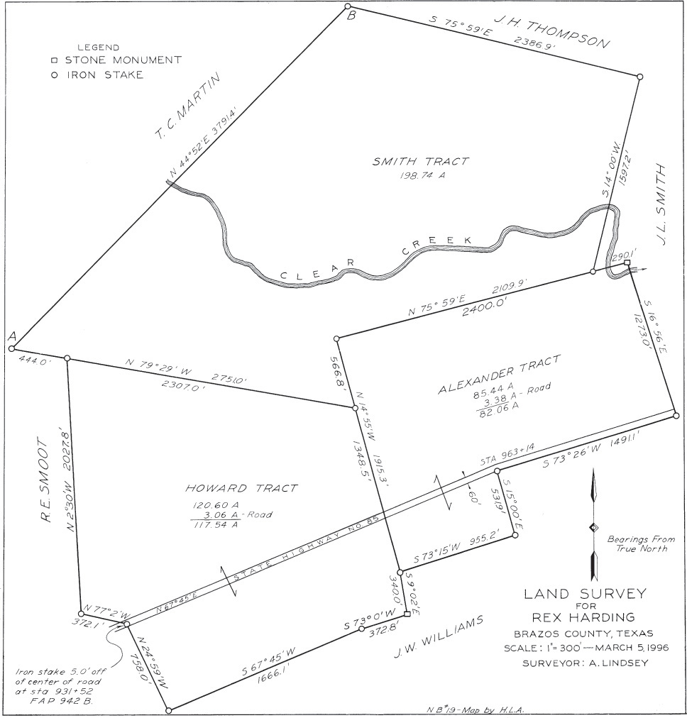
A traverse consists of a series of intersecting straight lines of accurately measured lengths. At the points of intersection, the deflection angles between adjacent lines are measured and recorded. From the starting point you can calculate rectangular coordinates of the other intersection points using trigonometry. A closed traverse is a closed polygon that allows you to check the accuracy of the surveyed information based on whether or not the last angle and distance meet back at the starting point of the loop. The land survey plat of Figure 19.1 shows a closed traverse.
Elevations are vertical distances above a common datum, or reference plane or point. The elevation of a point on the surface of the ground is usually determined by differential leveling from some other point of known elevation. Commonly, elevations are referenced to the mean sea level.
A profile is a line contained in a vertical plane, and it depicts the relative elevations of various points along the line. For example, if a vertical section were to be cut into the Earth, the top line of this section would represent the ground profile (Figure 19.2).
Contours are lines drawn on a map to locate, in the plan view, points of equal ground elevation. On a single contour line, therefore, all points have the same elevation (Figure 19.2).
Hatchures are short, parallel, or slightly divergent lines drawn in the direction of the slope. They are closely spaced on steep slopes and converge toward the tops of ridges and hills. Hatchures are shade lines used to show relief on older maps.
Monuments are special installations of stone or concrete to mark the locations of points accurately determined by precise surveying. It is intended that monuments be permanent or nearly so, and they are usually tied in by references to nearby natural features, such as trees and large boulders.
Cartography is the science or art of mapmaking.
Topographic maps (Figure 19.3) depict:
1. Water, including seas, lakes, ponds, rivers, streams, canals, and swamps;
2. Relief, or elevations, of mountains, hills, valleys, cliffs, and the like;
3. Culture, or human constructions, such as towns, cities, roads, railroads, airfields, and boundaries.

Hydrographic maps convey information concerning bodies of water, such as shoreline locations; relative elevations of points of lake, stream, or ocean beds; and sounding depths.
Cadastral maps are accurately drawn maps of cities and towns, showing property lines and other features that control property ownership.
Military maps contain information of military importance in the area represented.
Nautical maps and charts show navigational features and aids, such as locations of buoys, shoals, lighthouses and beacons, and sounding depths.
Aeronautical maps and charts show prominent landmarks, towers, beacons, and elevations for the use of air navigators.
Engineering maps are made for special projects as an aid to locations and construction.
Landscape maps are used in planning installations of trees, shrubbery, drives, and other garden features in the artistic design of area improvements.
Getting Information for Maps
A survey is the basis of all maps and topographic drawings. Several surveying methods are used to obtain the information necessary to make a map.
Most surveys use electronic survey instruments to measure distances and angles. To measure to a distant point, the surveyor aims the instrument toward the point, where a passive reflector or prism has been set. The instrument generates either a modulated infrared light signal focused into a narrow beam, or a laser beam, aimed directly at the reflector. When the reflector bounces the beam back to the aiming head, the beam’s travel time is measured electronically and directly converted into the distance to the point. One advantage of electronic measurement over the distance-taping method is that it is not necessary to stop traffic to take measurements. Electronic instruments measure distances of up to 4 mi with accuracies from .01′ to .03′, which is more than sufficient for topographic surveying. Figure 19.4 shows a Trimble VX spatial station. This type of instrument is often used to gather survey data.

Global positioning system (GPS) receivers calculate the receiver’s position by interpreting data received from four different satellites concurrently through a process called trilateration (which is similar to triangulation). Figure 19.5 shows a GPS satellite. Twenty-four satellites orbit the earth in a pattern called a GPS satellite constellation (see Figure 19.6). Each of these satellites broadcasts a signal that includes the precise time from the satellite’s onboard atomic clock. The distance to the satellite from the position of a GPS receiver can be calculated based on the time delay in receiving the signal. From any position on Earth a receiver should be able to locate four satellites and using trilateration calculate very accurately the position of the receiver on the surface of the Earth. Most modern maps of large areas are prepared using GPS positioning and satellite imagery.


19.6 GPS Satellite Constellation (Courtesy of Aerospace Corporation, http://www.aero.org.)
While GPS has revolutionized surveying, the vertical accuracy of GPS measurements (elevations) has not been as good as the horizontal accuracy (latitude and longitude). Knowledge of elevations is critical to surveyors, engineers, coastal managers, developers, and those who make resource or land-use management decisions.
Because forces such as sea level rise, subsidence (i.e., land sinking), and geological events constantly change the surface of the Earth, it is necessary to periodically resurvey areas to correct for changes. State and local governments spend tens of millions of dollars each year adjusting engineering projects that are continually affected by changing land surfaces, so a fast, yet accurate, method for determining elevations is needed. Height Modernization, which uses GPS in conjunction with other new and existing technologies to increase the accuracy of elevation measurements, is one such method.
Photogrammetry and satellite imagery are widely used for map surveying. They use actual photographs of the Earth’s surface and manufactured objects on the Earth. Aerial photogrammetry, via aircraft or satellite, is used for purposes such as governmental and commercial surveying, explorations, and property valuation. It has the advantage of being easy to use in difficult terrain with steep slopes, where ground surveying would be difficult or nearly impossible.
19.7 3D laser scanning solutions such as Trimble RealWorks allow you to integrate point data and extract measurements inside a 3D CAD environment. (Courtesy of Trimble Navigation Ltd.)
Taking photographs from ground stations with the axis of the camera lens nearly horizontal is called terrestrial photogrammetry. By combining the results of both aerial and terrestrial types of observations, it is possible to determine the relative positions of objects in a horizontal plane and their relative elevations.
Photogrammetry can be the basis of contour mapping as well as plan mapping. Generally, aerial photographs are used by forming a mosaic of photographs, which must overlap one another slightly. Photogrammetry offers the distinct advantage that a large area can be mapped from a single clear photograph. Photogrammetry can be used in connection with ground surveying by photographing control points already located on the ground by precise surveying.
For large land developments and large construction projects, new technologies for producing topographic maps have evolved. Some state highway departments and most engineering firms that specialize in surveying and mapping now make use of aerial photography with computers, terrain digitizers, stereoplotters, GIS, and various photo-laboratory techniques. In high volume work situations, expensive equipment may save enough time to justify its cost.
Laser distance meters typically calculate distance based on the difference in phase between the internal reference laser pulse and the external laser pulse reflected from the targeted object or a reflector plate attached to it. An example of this type of device is shown in Figure 19.8.

19.8 The Disto A8 Laser Distance Meter Allows Measurement of Distances up to 200 m (650′) with Precision of ±1.5 mm (.06″). (Courtesy of Leica Geosystems, Switzerland.)
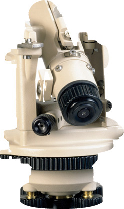
Optical mechanical systems are less used today. Before electronic measurement systems became affordable, an optical instrumental method called the stadia method was used in mapmaking. A stadia transit is an optical instrument used with a stadia rod. The instrument reading obtained by sighting visually on the rod and using a conversion factor, could be converted to distance. An example of this type of device is shown in Figure 19.9.
Short distances are ordinarily measured by steel tape, with driven stakes marking the points between field measurements.
Scaled measurements are made on rare occasions. In this method, distances are determined by measuring aerial photographs, when the scale is known.
For additional information, refer to publications such as the Manual of Surveying Instructions for the Survey of the Public Lands of the United States, prepared and published by the Bureau of Land Management (U.S. Government Printing Office, Washington, DC). Many governmental agencies also publicize information about maps and geographic data on the Web.
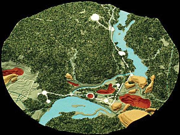
Rise of the Three Gorges Dam
Completed in 2009, the Three Gorges Dam is the world’s largest hydroelectric power generator and one of the few man-made structures so enormous that it’s visible to the naked eye from space.
The dam is built along the Yangtze River, the third largest in the world, stretching more than 3,900 miles across China. Historically, the river has been prone to massive flooding, overflowing its banks about once every 10 years. The dam is designed to improve flood control on the river and protect the 15 million people and 3.7 million acres of farmland in the Yangtze flood plains.
Observations from the NASA-built Landsat satellites provide an overview of the dam’s construction. The earliest data set, from 1987, shows the region prior to the start of construction. By 2000, construction along each riverbank was underway, but sediment-filled water still flowed through a narrow channel near the river’s south bank. The 2004 data shows development of the main wall and the partial filling of the reservoir, including numerous side canyons. By mid-2006, construction of the main wall was completed and a reservoir more than 2 mi (3 km) across had filled just upstream of the dam.

Satellite Imagery of the Three Gorges Dam (Courtesy of NASA.)
19.1 Symbols
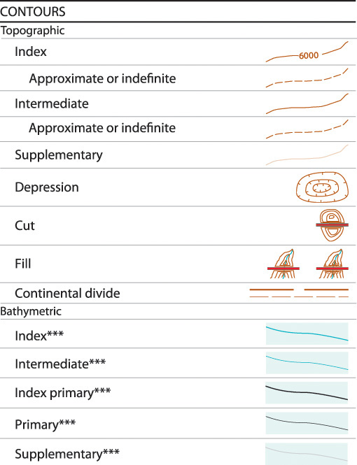
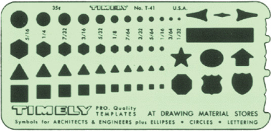
Various natural and human-made features are designated by special symbols. A list of the most commonly used map symbols is given in Appendix 32. Figure 19.10 shows an example of some commonly used symbols. You can find a full set on the Web at http://pubs.usgs.gov/tm/2006/11A02. Templates such as that shown in Figure 19.11 can save time in drawing map symbols by hand.
19.2 Bearings
The bearing of a line is its angle from magnetic north. Bearings are listed by referencing the angle the line makes departing from either the north or the south toward either the east or west. In Figure 19.12, the bearing for traverse line AB is N 44°52′ E, meaning that if you were standing at point A facing north, you would turn 44°52′ toward the east to face point B. (If you were at point B, you would use the opposite directions to face point A, facing south and turning 44°52′ toward the west.)
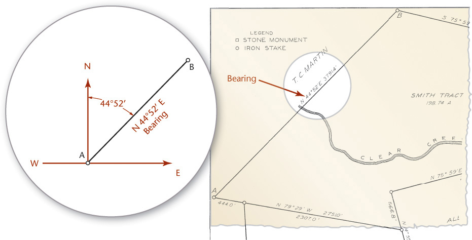
19.12 Bearings Specify an Angle and Direction from North or South toward East or West. The bearing N 44°52′ E means that if you were at point A facing north, you would turn 44°52′ toward the east to face point B.
Once the bearings of the lines of a traverse have been determined, the angles between them can be computed by adding or subtracting. Electronic survey instruments are used to calculate the bearings of lines, because compass readings are not accurate. Magnetic north and true north are not the same, and local magnetism may affect the position of the compass needle.
19.3 Elevation
If GPS is not used to provide elevation, an optical instrument called a level, equipped with a telescope for sighting long distances, can be used to determine differences in elevation in the field. The process is called differential leveling. When the instrument is leveled, the line of sight of its telescope is horizontal. A level rod, graduated in feet and decimals of feet, may be held on various points. Instrument readings of the rod then serve to determine the differences in elevations of the points.
19.4 Contours
Contours are map lines showing points of equal ground elevation. Figure 19.13 shows a comparison between a contour map and a satellite image taken from the TopoZone website.
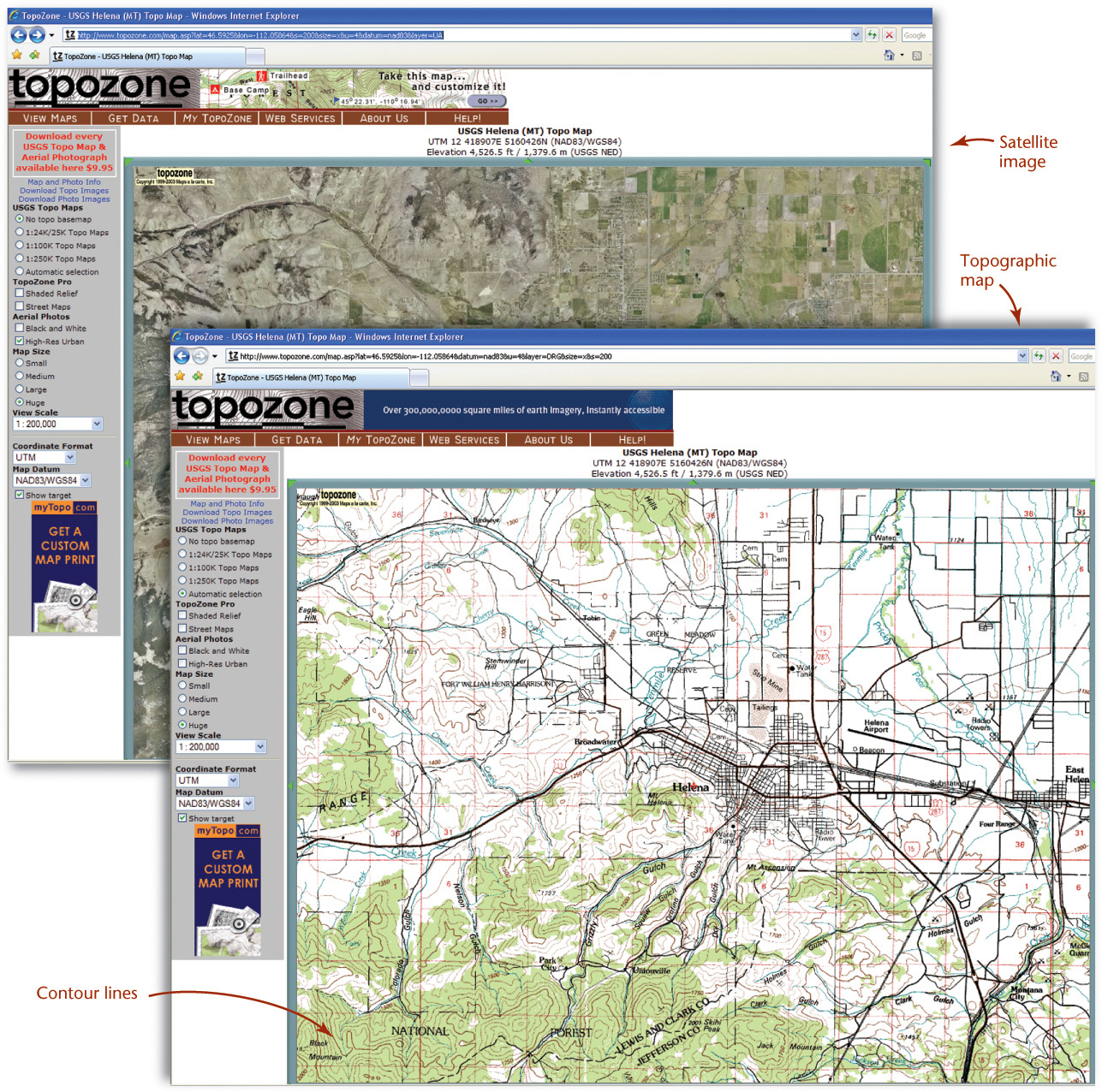
19.13 Topographic Map with Contours and Satellite Imagery (Courtesy of TopoZone at www.topozone.com)
A contour interval is the vertical distance between horizontal planes passing through successive contours. For example, in Figure 19.14 the contour interval is 10′. The contour interval should not change on any one map. It is customary to show every fifth contour by a line heavier than those representing intermediate contours.
For contour lines keep in mind:
• If extended far enough, every contour line will close.
• At streams, contours form Vs pointing upstream.
• Even spacing between successive contours means that the ground slopes uniformly.
• Uneven spacing between contours means that the slope changes frequently.
• Widely spaced contours indicate a gentle slope.
• Closely spaced contours indicate steep slopes.
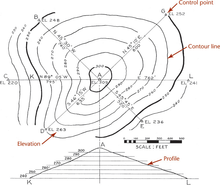
Interpolating Elevation Data
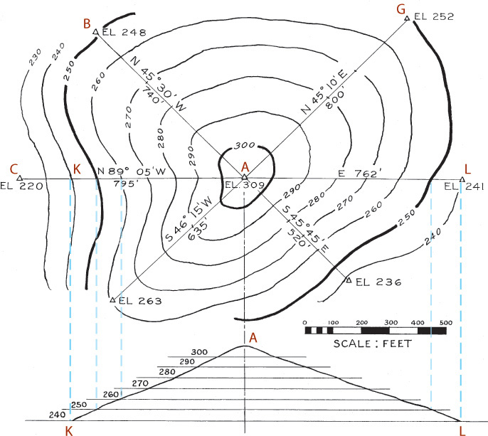
Locations of points on contour lines are determined by interpolation. In Figure 19.14, the locations and elevations of seven control points have been determined. The goal is to draw the contour lines assuming the slope of the surface of the ground is uniform between station A and the six adjacent stations, using a contour interval of 10′. The locations of the intersections of the contour lines with the straight lines joining the point A and the six adjacent points, were calculated as follows.
The horizontal distance between stations A and B is 740′. The difference in elevation of those stations is 61′. The difference in elevation of station A and contour 300 is 9′; therefore, contour 300 crosses line AB at a distance from station A of 9/61 of 740, or 109.1′. Contour 290 crosses the line AB at a distance from contour 300 of 10/61 of 740, or 121.3′. This 121.3′ distance between contour lines is constant along the line AB and can be measured without more calculations.
You can interpolate points where the contours cross the other lines of the survey the same way. After interpolating the elevations you can draw the contour lines through points of equal elevation as shown.
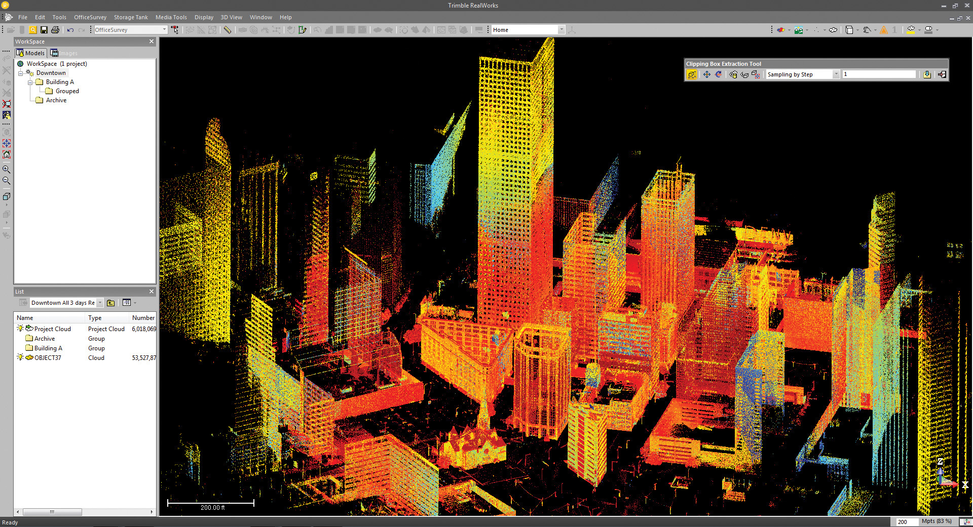
After contours have been plotted, you can draw a profile of the ground line in any direction. In Figure 19.14, the profile of line KAL is shown in the lower or front view. It is customary, as shown here, to draw the profile using an exaggerated vertical scale to emphasize the varying slopes. Laser scanning combined with increasingly accurate GPS satellite data allows highly detailed depiction of terrain such as that shown in Figure 19.15.

19.15 Elevation-Based Rendering. Trimble RealWorks software will display the point cloud captured in a 3D scan using color to indicate elevation. (Courtesy of Trimble Navigation Ltd.)
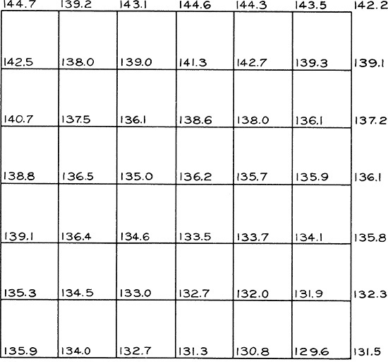
Contour lines may be plotted from recorded elevations of points on the ground, as in Figure 19.16a. This figure illustrates a checkerboard survey, in which lines are drawn at right angles to each other, dividing the survey into 100′ squares, and where elevations have been measured at the corners of the squares. The contour interval is taken as 2′, and the slope of the ground between adjacent stations is assumed to be uniform.
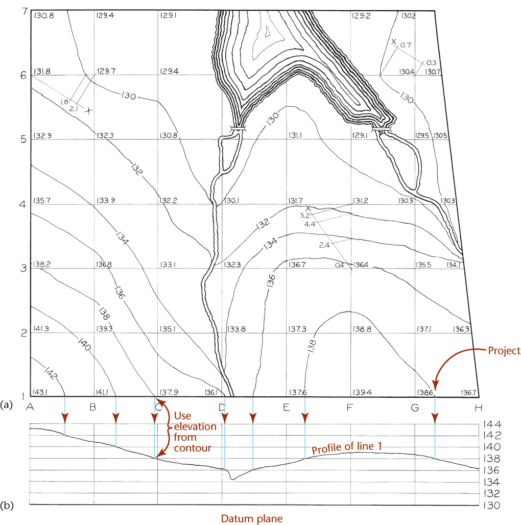
The points where the contour lines cross the survey lines can be located approximately by inspection, by graphical methods, or by the numerical method explained for Figure 19.14.
You can also find the points of intersection that contour lines make with survey lines by constructing a profile of each line of the survey, as shown for line 1 in Figure 19.16b. Draw horizontal lines at elevations where you want to show contours. The points where the profile line intersects these horizontal lines are the elevations of points where corresponding contour lines cross the survey line 1. These can be projected upward, as shown, to locate these points.
The profile of any line can be constructed from the contour map by the converse of the process just described.
3D Terrain Models
Electronic survey data containing elevations can often be downloaded directly to 3D terrain modeling software. Most of these software solutions produce a surface model of the terrain formed of many small triangles and are thus called a Triangulated Irregular Network, or TIN. Contours, profiles, cut-and-fill calculations, and other information can be generated semiautomatically from the TIN. An example is shown in Figure 19.17.
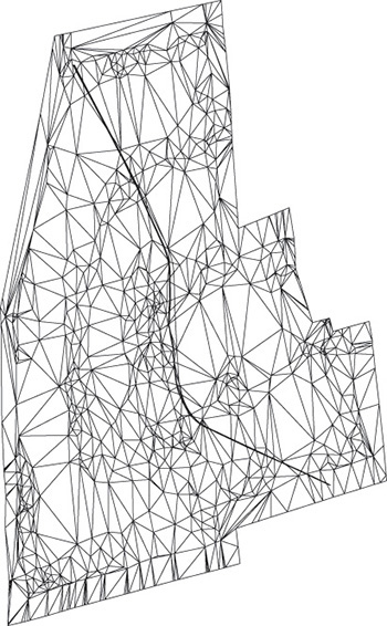
19.17 TIN 3D Terrain Model Produced in Autodesk Civil 3D (Used with permission of Autodesk, Inc. All rights reserved.)
19.5 City Maps
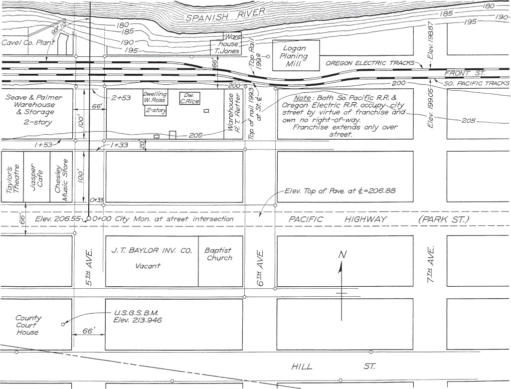
The particular use of a map determines what features are to be shown. Maps of city areas may be put to many uses. Figure 19.18, a city plan for location of new road construction, shows only those features of importance to the location and construction of the road. The transit line starts at the centerline intersection of Park St. and 5th Ave., and it is marked as station 0 + 00. From here it extends north over the railroad yard to cross the river. Features near the transit line, such as buildings, are shown and identified by name. Street widths are important and are shown. Contour lines between the railroad yard and the river indicate the steeply sloping terrain.
Subdivision Plats
Maps perform an important function for those who plan the layout of lots and streets. For example, Figure 19.19a shows an original layout of these features for a new residential area. An examination of the contours will show that this layout is not satisfactory, since the directions of the streets do not fit the natural ground slopes. Streets should be arranged so that the subdivision can be entered from a low point and so that a maximum number of lots will be above street grade. The layout in Figure 19.19b is a decided improvement, for in it the streets curve to fit the topography, and the entrance is located at a low point.
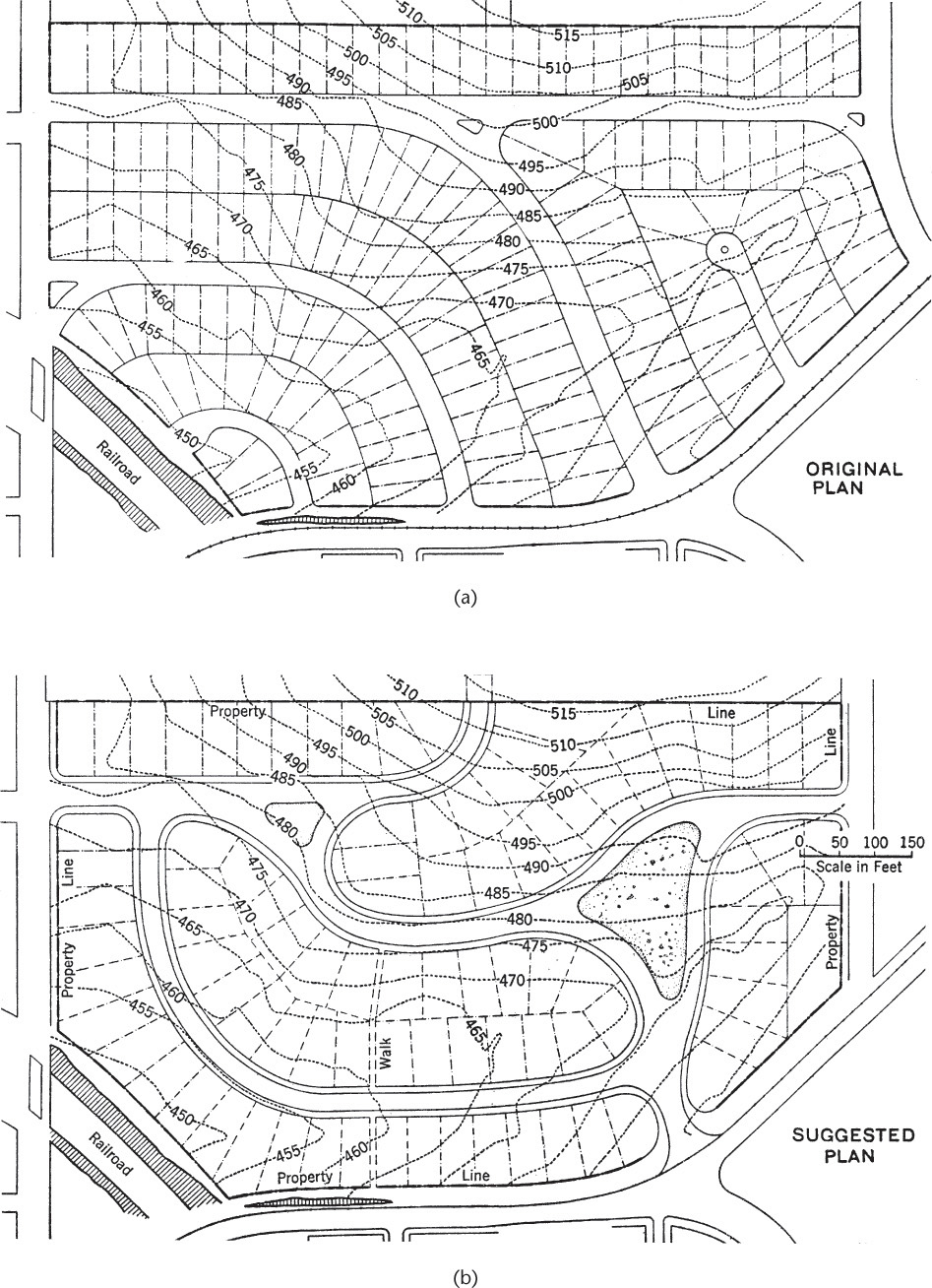
19.19 Adjustment of Streets to Topography (From Land Subdivision, ASCE Manual No. 16 of Engineering Practice, with permission from ASCE.)
Uses for Subdivision Plats
Utilities and other information are often referenced to locations from subdivision plats. A subdivision plat showing the locations of above-ground and underground power is shown in Figure 19.20. Subdivision plats are recorded legal documents, and they are often available from county clerks and recorders’ offices. These drawings are used as reference for property boundaries, for landscape development, and other uses.

19.20 Above-ground and underground power is located from subdivision plats. (Courtesy of Golden Valley Electric Association.)
Landscape Drawings
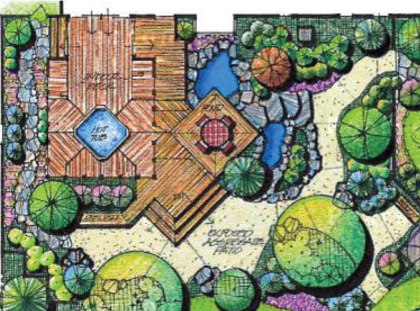
Maps have a definite use in landscape planning. Figure 19.21 is a landscape drawing showing a proposed layout of a deck, water feature, and trees for beautification of an outdoor space.
19.6 Structure Location Plans
Maps are used to plan construction projects and locate construction features so they fit the topography of the area. A project location plan for a dam is shown in Figure 19.22. This map shows the important natural features, contours, a plan view of the structure, and a cross section through Hoover Dam.

19.22 Plan for Hoover Dam (From Treatise on Dams. Courtesy of U.S. Dept. of the Interior, Bureau of Reclamation.)
To show the complete construction drawings for a large bridge project may take hundreds of drawings, but one of the most important early drawings is a general arrangement plan and elevation in the form of a line diagram. Figure 19.23 is an example—a plan and elevation of a large bridge structure.

19.7 Highway Plans
Before highway construction starts, it is necessary to plan the horizontal and vertical location and alignments. Commonly, both the plan view and profile are drawn on the same sheet, as in Figure 19.24.
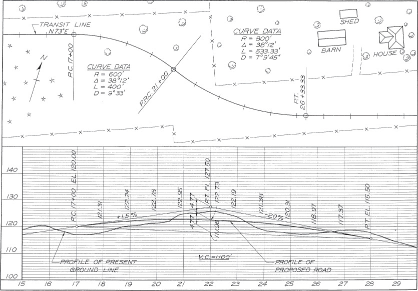
The topographical plan at the top of Figure 19.24 shows such features as trees, fences, and farmhouses along the right of way. The transit line, locating the centerline of the new road, is drawn with stations located every 100 ft, 50 m, or some other convenient spacing. Data for creating the horizontal curves in the field are calculated and listed on the drawing.
Reading the information on the drawing, notice that the point of curve (P.C.) at station 17 + 00 is the point at which the line begins to curve with a 600′ radius, for a curve length of 400′. The central angle is 38°12′, and the degree of curve (the angle subtended by a 100′ chord) is shown as 9°33′. The reverse curve of 800′ radius begins at station 21 + 00. Note also the North point and the bearing N 73° E of the transit line.
The vertical alignment is shown in profile below the plan view. Note the station numbers listed below the profile. The scale of this view is larger in the vertical than in the horizontal direction to exaggerate the elevations so they show easily. The existing ground profile along the centerline of the road is shown, as well as the profile of the proposed vertical alignment. The symbol P. I. denotes the point of intersection of the grade lines, and grade slopes are given in percentages. A 1% grade would rise vertically 1′ in each 100′ of horizontal distance. Station 22 + 00, therefore, is the intersection point of an upgrade of 1.5% and a downgrade of –2%.
To provide a smooth transition between these grades, a vertical curve (V.C.) of 1100′ length was used. This curve is parabolic and tangent to grade at stations 17 + 00 and 28 + 00. The straight line joining these points has an elevation 117.96′ directly below the P. I. At this point the parabolic curve must pass through the midpoint of the vertical distance, at a height of 4.77′ below the P. I.
The final profile elevations are given in Figure 19.24. Calculations are given in Table 19.1.
Table 19.1 Calculation of Vertical Curve Elevations
Station |
Tangent Elevations |
Ordinate |
Curve Elevations |
18 |
121.50 |
.19* |
121.31 |
19 |
123.00 |
.76 |
122.24 |
20 |
124.50 |
1.72 |
122.78 |
21 |
126.00 |
3.05 |
122.95 |
22 |
127.50 |
4.77 |
122.73 |
23 |
125.50 |
3.31 |
122.19 |
24 |
123.50 |
2.12 |
121.38 |
25 |
121.50 |
1.19 |
120.31 |
26 |
119.50 |
.53 |
118.97 |
27 |
117.50 |
.13 |
117.37 |
Tip
Ordinates to parabolas, measured from tangents, are proportional to the squares of the horizontal distances from the points of tangency. Therefore, it is possible to calculate the elevations of points along the curve by first determining the grade elevations and then subtracting the parabolic curve ordinates.
CAD at Work: Contour Maps from 3D Data
CAD software like Autodesk’s Civil 3D allows you to create contour maps by entering site data such as that shown in Figure A. Data can even be downloaded directly into the CAD software from a total station survey instrument.

(A) Autodesk Civil 3D software provides tools to generate contour maps from survey data. (Autodesk screen shots reprinted courtesy of Autodesk, Inc.)
Using Civil 3D software, you can show point descriptions, contour lines, grid lines, and features such as bodies of water or structures and produce topographic pictorial drawings.
Planners are able to lay out roads and subdivisions using specialized software features that provide the contractor with earthwork calculations for individual lots or the entire site.
The same survey data that produce contour maps can be used to produce profiles like those shown in Figure B. Profiles generated from a TIN can be used for earthwork calculations. Street intersections and features such as cul-de-sacs can be automatically generated.
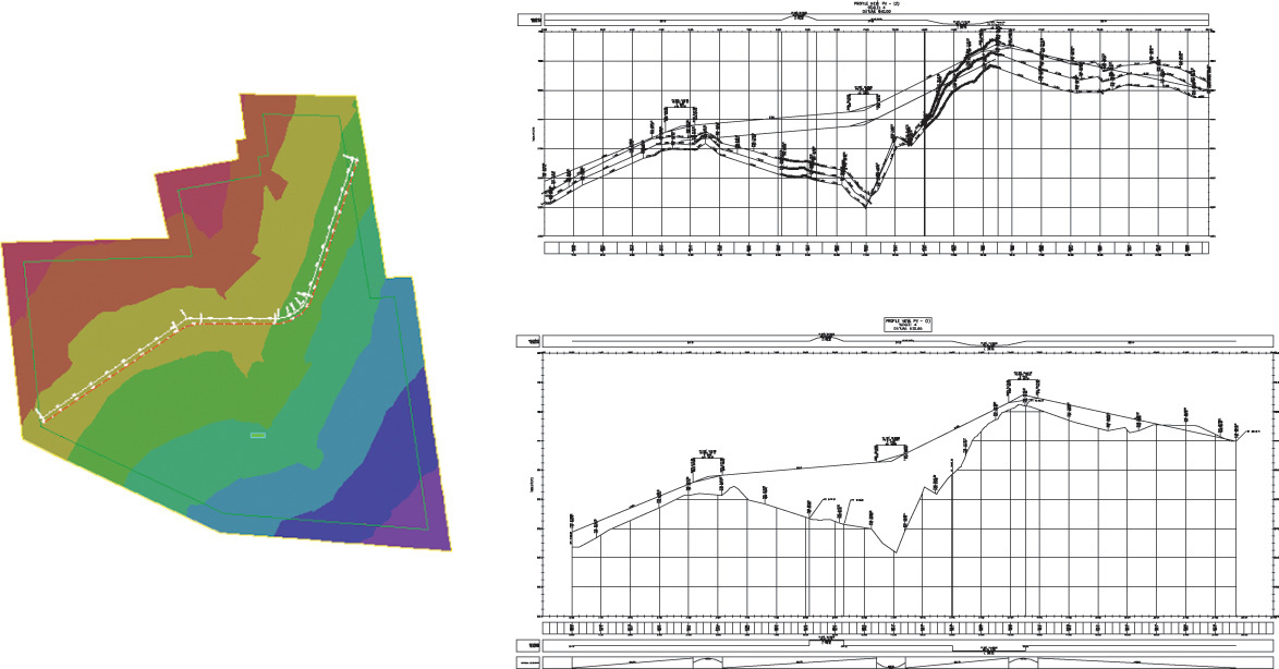
(B) Profiles can be generated across any alignment once the TIN for site has been created. The profiles shown above are from alignments shown in the colored contour map at left. (Autodesk screen shots reprinted courtesy of Autodesk, Inc.)
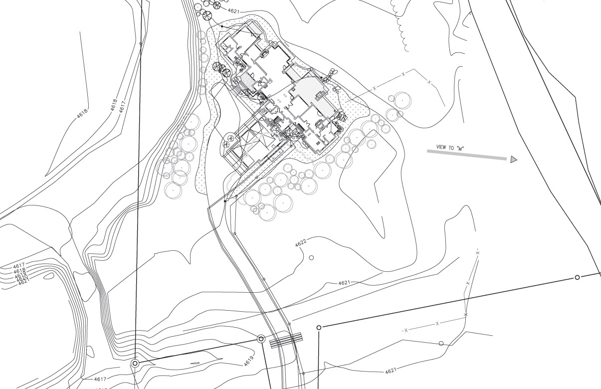
This portion of a site plan shows contours, lot boundaries, utility easement, and the primary view directions. (Courtesy of Locati Architects.)
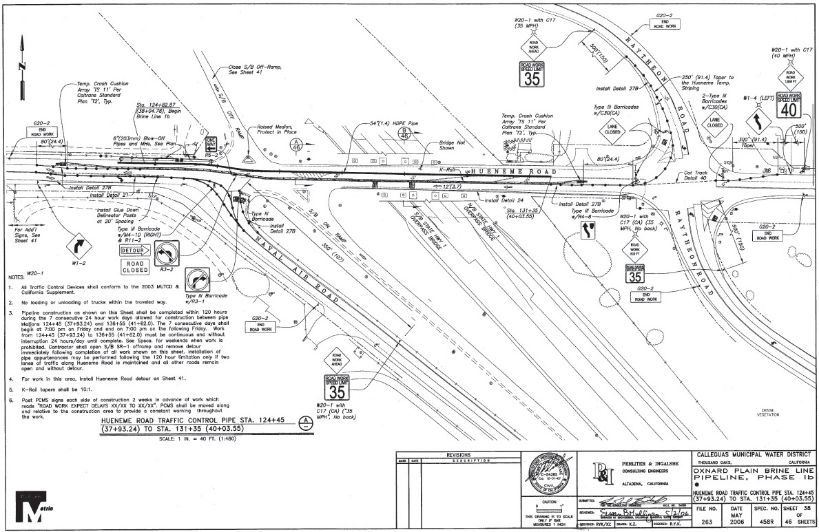
Highway signage and barricades, along with trees, shrubs, and fences, are located on this pipeline construction traffic control drawing. (Courtesy of Perliter and Ingalsbe Consulting Engineers and Calleguas Municipal Water District.)
Global Positioning System (GPS)
Photogrammetry and Satellite Imagery
Quadrangle
Chapter Summary
• Topographic drawings represent three dimensions on a 2D plan view.
• Land surveys denote the boundaries of tracts of land. Boundaries are defined by bearing and length.
• Contour lines are used to show elevation on a plan drawing. Each contour line represents one elevation level. Closely spaced contour lines indicate a steep slope. Widely spaced contour lines indicate a flatter slope.
• A profile drawing of elevation is created by drawing a cutting-plane datum on the plan view and transferring distances and elevation from the plan to the profile drawing. Profile drawings are often used to determine cut-and-fill slopes for roadways and railways.
• Land subdivision drawings show roads, property boundaries, and major landscape landmarks such as parks, streams, buildings, and large trees.
• Computer graphics workstations can model 3D surfaces from satellite photographs. Computers model surfaces by creating a wireframe structure and then applying solid color contours to the wireframe surface.
Review Questions
1. What is the purpose of a plat drawing? Is it a plan or an elevation?
2. What is the topographic notation for a plat boundary that runs exactly east and west for 1503.4′?
3. What are the lines that indicate elevation on a topographic map?
4. What is the purpose of a profile drawing?
5. If contour lines are very close together, is the slope steep or gentle?
Chapter Exercises
The following problems are given to afford practice in topographic drawing. They may be completed by using either traditional drawing methods or a CAD program. The drawings are designed for a size B or A3 sheet. The position and arrangement of the titles should conform approximately to those of Figure 19.1.
Exercise 19.1 Draw symbols of six of the common natural surface features (streams, lakes, etc.) and six of the common development features (roads, buildings, etc.) shown in Appendix 32.
Exercise 19.2 Draw, to assigned horizontal and vertical scales, profiles of any three of the six lines shown in Figure 19.14.
Exercise 19.3 Assuming the slope of the ground to be uniform and assuming a horizontal scale of 1″ = 200′ and a contour interval of 5′, plot, by interpolation, the contours of Figure 19.14.
Exercise 19.4 Using the elevations shown in Figure 19.16a and a contour interval of 1′, plot the contours to any convenient horizontal and vertical scales, and draw profiles of lines 3 and 5 and of any two lines perpendicular to them. Check, graphically, the points in which the contours cross these lines.
Exercise 19.5 Using a contour interval of 1′ and a horizontal scale of 1″ = 100′, plot the contours from the elevations given above at 100′ stations. Check, graphically, the points in which the contours cross one of the horizontal lines and one of the vertical lines, using a vertical scale of 1″ = 10′. Sketch, approximately, the drainage channels.
Exercise 19.6 Use CAD to draw a plat of the survey shown in Figure 19.1. If the drawing is accurate, the plat will close. Plot your final drawing on as large a sheet as practical. Determine a standard scale at which to show the drawing. Make sure the text labeling your drawing lines appears legible and at a standard height.
Exercise 19.7 Draw a topographic map of a country estate similar to that shown in Figure 19.3.
Exercise 19.8 Calculate profile elevations for a vertical curve 800′ long to join grades of +3.00% and –3.00%. Assume grade elevations at points of tangency to be 100.00′.