Local Receptive Fields

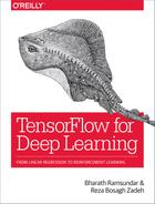
The local receptive field concept originates in neuroscience, where the receptive field of a neuron is the part of the body’s sensory perception that affects the neuron’s firing. Neurons have a certain field of “view” as they process sensory input that the brain sees. This field of view is traditionally called the local receptive field. This “field of view” could correspond to a patch of skin or to a segment of a person’s visual field. Figure 6-1 illustrates a neuron’s local receptive field.

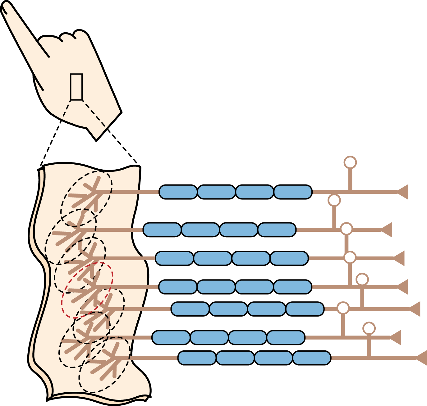
Figure 6-1. An illustration of a neuron’s local receptive field.

Convolutional architectures borrow this latter concept with the computational notion of “local receptive fields.” Figure 6-2 provides a pictorial representation of the local receptive field concept applied to image data. Each local receptive field corresponds to a patch of pixels in the image and is handled by a separate “neuron.” These “neurons” are directly analogous to those in fully connected layers. As with fully connected layers, a nonlinear transformation is applied to incoming data (which originates from the local receptive image patch).

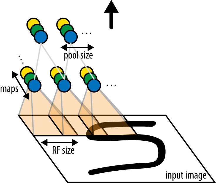
Figure 6-2. The local receptive field (RF) of a “neuron” in a convolutional network.

A layer of such “convolutional neurons” can be combined into a convolutional layer. This layer can viewed as a transformation of one spatial region into another. In the case of images, one batch of images is transformed into another by a convolutional layer. Figure 6-3 illustrates such a transformation. In the next section, we will show you more details about how a convolutional layer is constructed.

Figure 6-3. A convolutional layer performs an image transformation.

It’s worth emphasizing that local receptive fields don’t have to be limited to image data. For example, in stacked convolutional architectures, where the output of one convolutional layer feeds into the input of the next, the local receptive field will correspond to a “patch” of processed feature data.

Convolutional Kernels

In the last section, we mentioned that a convolutional layer applies nonlinear function to a local receptive field in its input. This locally applied nonlinearity is at the heart of convolutional architectures, but it’s not the only piece. The second part of the convolution is what’s called a “convolutional kernel.” A convolutional kernel is just a matrix of weights, much like the weights associated with a fully connected layer. Figure 6-4 diagrammatically illustrates how a convolutional kernel is applied to inputs.

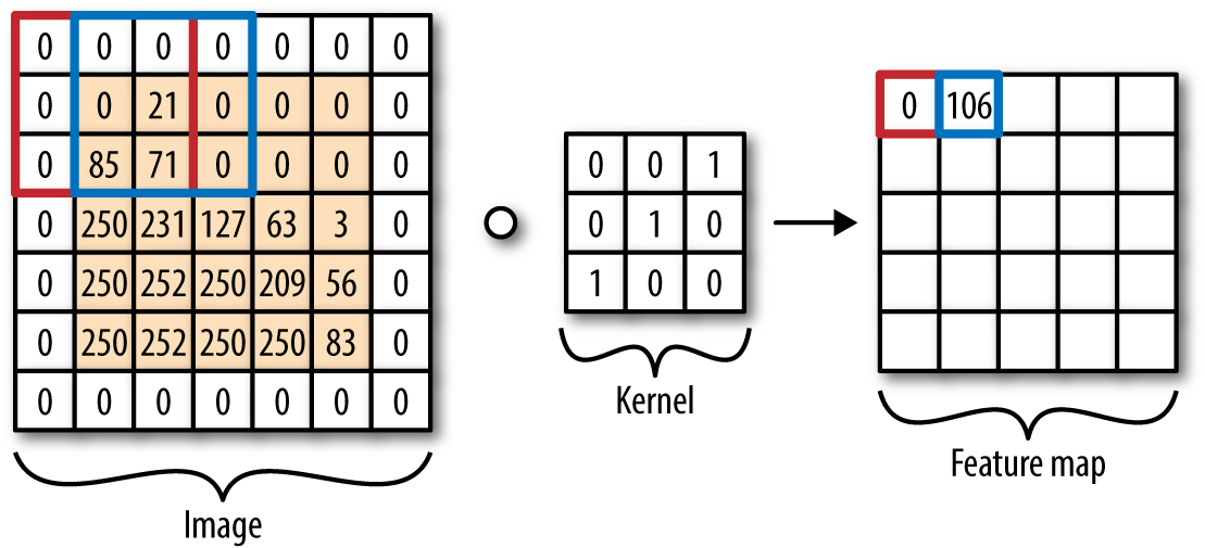
Figure 6-4. A convolutional kernel is applied to inputs. The kernel weights are multiplied elementwise with the corresponding numbers in the local receptive field and the multiplied numbers are summed. Note that this corresponds to a convolutional layer without a nonlinearity.

The key idea behind convolutional networks is that the same (nonlinear) transformation is applied to every local receptive field in the image. Visually, picture the local receptive field as a sliding window dragged over the image. At each positioning of the local receptive field, the nonlinear function is applied to return a single number corresponding to that image patch. As Figure 6-4 demonstrates, this transformation turns one grid of numbers into another grid of numbers. For image data, it’s common to label the size of the local receptive field in terms of the number of pixels on each size of the receptive field. For example, 5 × 5 and 7 × 7 local receptive field sizes are commonly seen in convolutional networks.

What if we want to specify that local receptive fields should not overlap? The way to do this is to alter the stride size of the convolutional kernel. The stride size controls how the receptive field is moved over the input. Figure 6-4 demonstrates a one-dimensional convolutional kernel, with stride sizes 1 and 2, respectively. Figure 6-5 illustrates how altering the stride size changes how the receptive field is moved over the input.

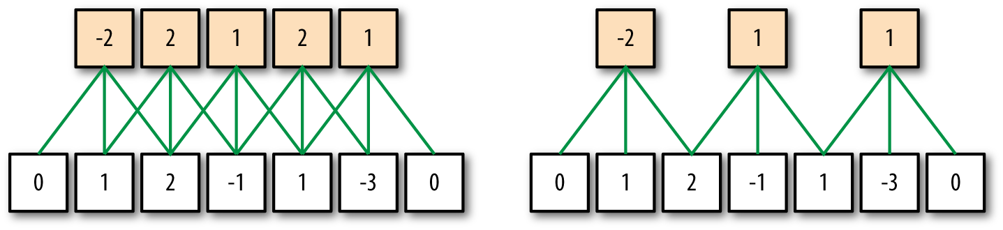
Figure 6-5. The stride size controls how the local receptive field “slides” over the input. This is easiest to visualize on a one-dimensional input. The network on the left has stride 1, while that on the right has stride 2. Note that each local receptive field computes the maximum of its inputs.

Now, note that the convolutional kernel we have defined transforms a grid of numbers into another grid of numbers. What if we want more than one grid of numbers output? It’s easy enough; we simply need to add more convolutional kernels for processing the image. Convolutional kernels are also called filters, so the number of filters in a convolutional layer controls the number of transformed grids we obtain. A collection of convolutional kernels forms a convolutional layer.

Pooling Layers

In the previous section, we introduced the notion of convolutional kernels. These kernels apply learnable nonlinear transformations to local patches of inputs. These transformations are learnable, and by the universal approximation theorem, capable of learning arbitrarily complex input transformations on local patches. This flexibility gives convolutional kernels much of their power. But at the same time, having many learnable weights in a deep convolutional network can slow training.

Instead of using a learnable transformation, it’s possible to instead use a fixed nonlinear transformation in order to reduce the computational cost of training a convolutional network. A popular fixed nonlinearity is “max pooling.” Such layers select and output the maximally activating input within each local receptive patch. Figure 6-6 demonstrates this process. Pooling layers are useful for reducing the dimensionality of input data in a structured fashion. More mathematically, they take a local receptive field and replace the nonlinear activation function at each portion of the field with the max (or min or average) function.

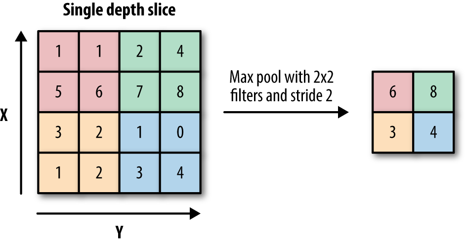
Figure 6-6. An illustration of a max pooling layer. Notice how the maximal value in each colored region (each local receptive field) is reported in the output.

Pooling layers have become less useful as hardware has improved. While pooling is still useful as a dimensionality reduction technique, recent research tends to avoid using pooling layers due to their inherent lossiness (it’s not possible to back out of pooled data which pixel in the input originated the reported activation). Nonetheless, pooling appears in many standard convolutional architectures so it’s worth understanding.

Constructing Convolutional Networks

A simple convolutional architecture applies a series of convolutional layers and pooling layers to its input to learn a complex function on the input image data. There are a lot of details in forming these networks, but at its heart, architecture design is simply an elaborate form of Lego stacking. Figure 6-7 demonstrates how a convolutional architecture might be built up out of constituent blocks.

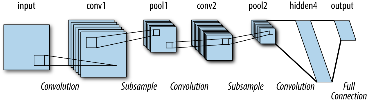
Figure 6-7. An illustration of a simple convolutional architecture constructed out of stacked convolutional and pooling layers.

Dilated Convolutions

Dilated or atrous convolutions are a newly popular form of convolutional layer. The insight here is to leave gaps in the local receptive field for each neuron (atrous means a trous, or “with holes” in French). The basic concept is an old one in signal processing that has recently found some good traction in the convolutional literature.

The core advantage to the atrous convolution is the increase in visible area for each neuron. Let’s consider a convolution architecture whose first layer is a vanilla convolutional with 3 × 3 local receptive fields. Then a neuron one layer deeper in the architecture in a second vanilla convolutional layer has receptive depth 5 × 5 (each neuron in a local receptive field of the second layer itself has a local receptive field in the first layer). Then, a neuron two layers deeper has receptive view 7 × 7. In general, a neuron N layers within the convolutional architecture has receptive view of size (2N + 1) × (2N + 1). This linear growth in receptive view is fine for smaller images, but quickly becomes a liability for large images.

The atrous convolution enables exponential growth in the visible receptive field by leaving gaps in its local receptive fields. A “1-dilated” convolution leaves no gaps, while a “2-dilated” convolution leaves one gap between each local receptive field element. Stacking dilated layers leads to exponentially increasing local receptive field sizes. Figure 6-8 illustrates this exponential increase.

Dilated convolutions can be very useful for large images. For example, medical images can stretch thousands of pixels in every dimension. Creating vanilla convolutional networks that have global understanding could require unreasonably deep networks. Using dilated convolutions could enable networks to better understand the global structure of such images.

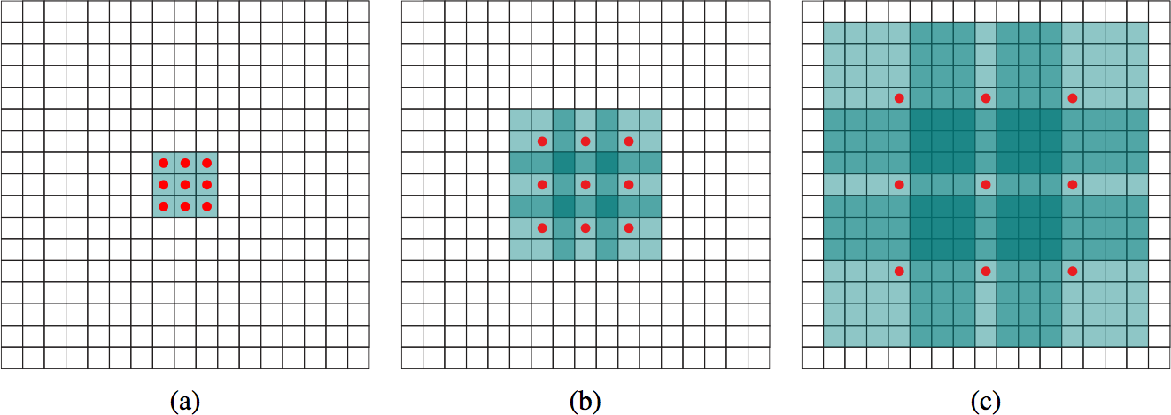
Figure 6-8. A dilated (or atrous) convolution. Gaps are left in the local receptive field for each neuron. Diagram (a) depicts a 1-dilated 3 × 3 convolution. Diagram (b) depicts the application of a 2-dilated 3 × 3 convolution to (a). Diagram (c) depicts the application of a 4-dilated 3 × 3 convolution to (b). Notice that the (a) layer has receptive field of width 3, the (b) layer has receptive field of width 7, and the (c) layer has receptive field of width 15.

Object Detection and Localization

Object detection is the task of detecting the objects (or entities) present in a photograph. Object localization is the task of identifying where in the image the objects exist and drawing a “bounding box” around each occurrence. Figure 6-9 demonstrates what detection and localization on standard images looks like.

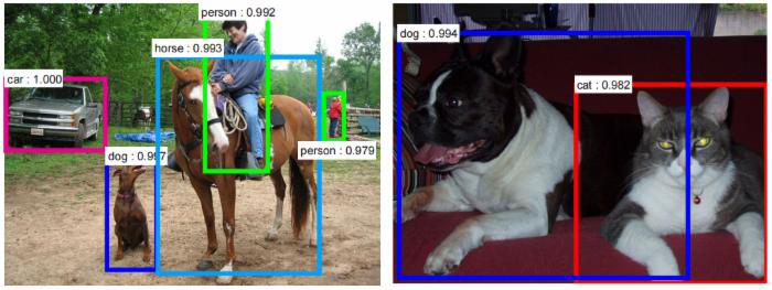
Figure 6-9. Objects detected and localized with bounding boxes in some example images.

Why is detection and localization important? One very useful localization task is detecting pedestrians in images taken from a self-driving car. Needless to say, it’s extremely important that a self-driving car be able to identify all nearby pedestrians. Other applications of object detection could be used to find all instances of friends in photos uploaded to a social network. Yet another application could be to identify potential collision dangers from a drone.

This wealth of applications has made detection and localization the focus of tremendous amounts of research activity. The ILSVRC challenge mentioned multiple times in this book focused on detecting and localizing objects found in the ImagetNet collection.

Image Segmentation

Image segmentation is the task of labeling each pixel in an image with the object it belongs to. Segmentation is related to object localization, but is significantly harder since it requires precisely understanding the boundaries between objects in images. Until recently, image segmentation was often done with graphical models, an alternate form of machine learning (as opposed to deep networks), but recently convolutional segmentations have risen to prominence and allowed image segmentation algorithms to achieve new accuracy and speed records. Figure 6-10 displays an example of image segmentation applied to data for self-driving car imagery.

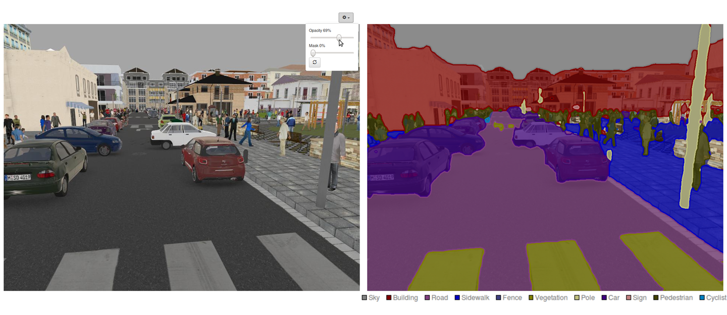
Figure 6-10. Objects in an image are “segmented” into various categories. Image segmentation is expected to prove very useful for applications such as self-driving cars and robotics since it will enable fine-grained scene understanding.

Graph Convolutions

The convolutional algorithms we’ve shown you thus far expect rectangular tensors as their inputs. Such inputs could come in the form of images, videos, or even sentences. Is it possible to generalize convolutions to apply to irregular inputs?

The fundamental idea underlying convolutional layers is the notion of a local receptive field. Each neuron computes upon the inputs in its local receptive field, which typically constitute adjacent pixels in an image input. For irregular inputs, such as the undirected graph in Figure 6-11, this simple notion of a local receptive field doesn’t make sense; there are no adjacent pixels. If we can define a more general local receptive field for an undirected graph, it stands to reason that we should be able to define convolutional layers that accept undirected graphs.

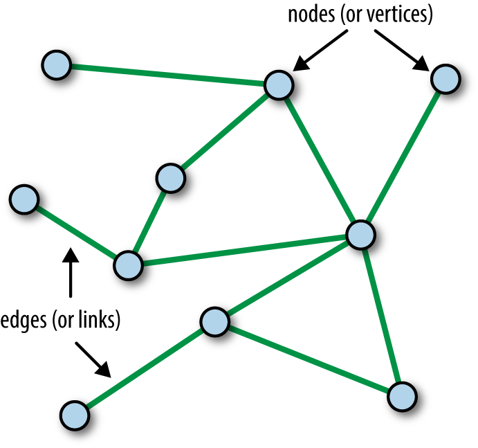
Figure 6-11. An illustration of an undirected graph consisting of nodes connected by edges.

As Figure 6-11 shows, a graph is made up of a collection of nodes connected by edges. One potential definition of a local receptive field might be to define it to constitute a node and its collection of neighbors (where two nodes are considered neighbors if they are connected by an edge). Using this definition of local receptive fields, it’s possible to define generalized notions of convolutional and pooling layers. These layers can be assembled into graph convolutional architectures.

Where might such graph convolutional architectures prove useful? In chemistry, it turns out molecules can be modeled as undirected graphs where atoms form nodes and chemical bonds form edges. As a result, graph convolutional architectures are particularly useful in chemical machine learning. For example, Figure 6-12 demonstrates how graph convolutional architectures can be applied to process molecular inputs.

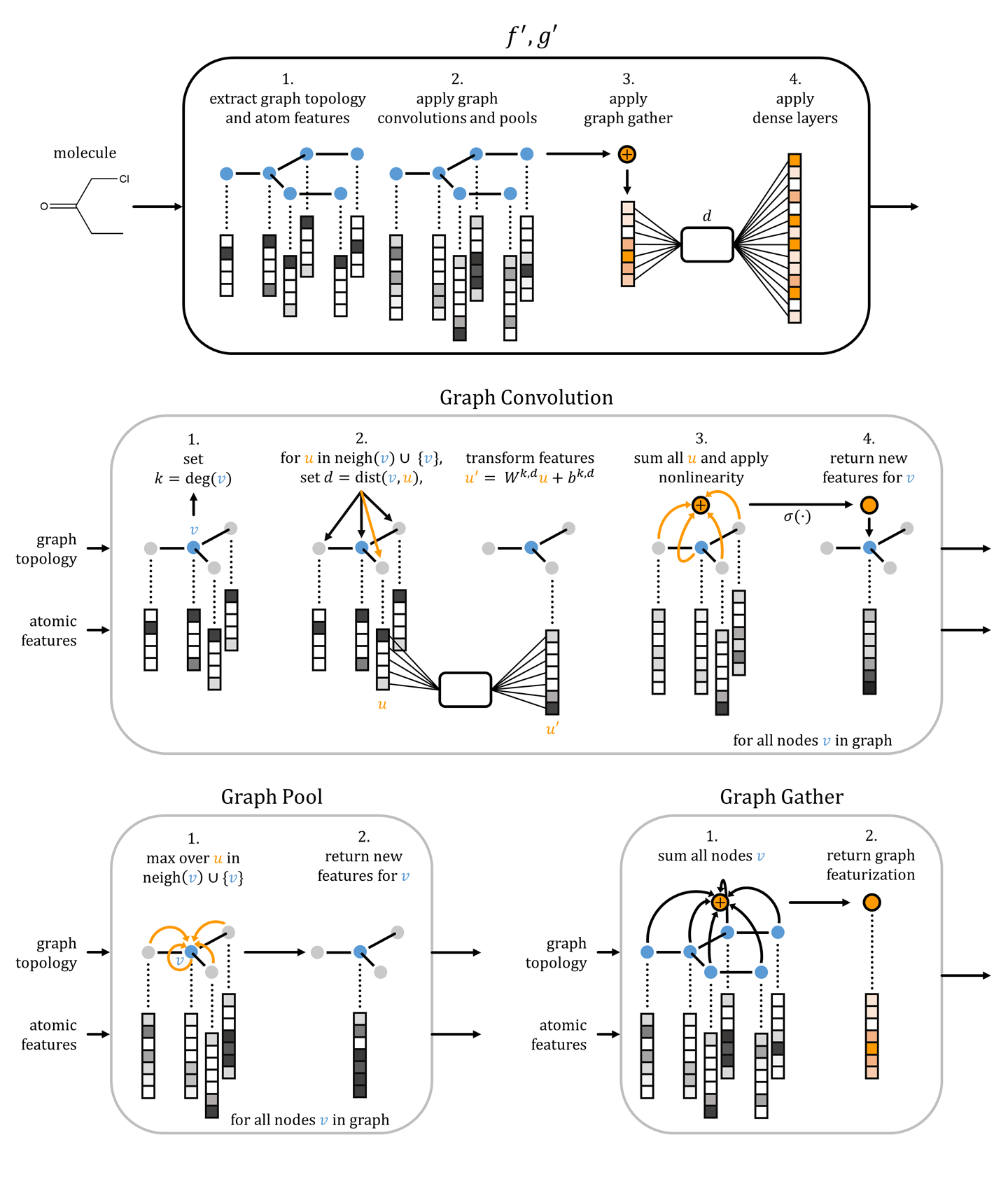
Figure 6-12. An illustration of a graph convolutional architecture processing a molecular input. The molecule is modeled as an undirected graph with atoms forming nodes and chemical bond edges. The “graph topology” is the undirected graph corresponding to the molecule. “Atom features” are vectors, one per atom, summarizing local chemistry. Adapted from “Low Data Drug Discovery with One-Shot Learning.”

Generating Images with Variational Autoencoders

The applications we’ve described thus far are all supervised learning problems. There are well-defined inputs and outputs, and the task remains (using a convolutional network) to learn a sophisticated function mapping input to output. Are there unsupervised learning problems that can be solved with convolutional networks? Recall that unsupervised learning requires “understanding” the structure of input datapoints. For image modeling, a good measure of understanding the structure of input images is being able to “sample” new images that come from the input distribution.

What does “sampling” an image mean? To explain, let’s suppose we have a dataset of dog images. Sampling a new dog image requires the generation of a new image of a dog that is not in the training data! The idea is that we would like a picture of a dog that could have reasonably been included with the training data, but was not. How could we solve this task with convolutional networks?

Perhaps we could train a model to take in word labels like “dog” and predict dog images. We might possibly be able to train a supervised model to solve this prediction problem, but the issue remains that our model could generate only one dog picture given the input label “dog.” Suppose now that we could attach a random tag to each dog—say “dog3422” or “dog9879.” Then all we’d need to do to get a new dog image would be to attach a new random tag, say “dog2221,” to get out a new picture of a dog.

Variational autoencoders formalize these intuitions. Variational autoencoders consist of two convolutional networks: the encoder and decoder network. The encoder network is used to transform an image into a flat “embedded” vector. The decoder network is responsible for transforming the embedded vector into images. Noise is added to ensure that different images can be sampled by the decoder. Figure 6-13 illustrates a variational autoencoder.

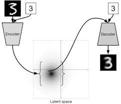
Figure 6-13. A diagrammatic illustration of a variational autoencoder. A variational autoencoder consists of two convolutional networks, the encoder and decoder.

There are more details involved in an actual implementation, but variational autoencoders are capable of sampling images. However, naive variational encoders seem to generate blurry image samples, as Figure 6-14 demonstrates. This blurriness may be because the L² loss doesn’t penalize image blurriness sharply (recall our discussion about L² not penalizing small deviations). To generate crisp image samples, we will need other architectures.

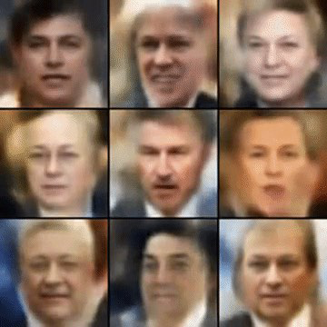
Figure 6-14. Images sampled from a variational autoencoder trained on a dataset of faces. Note that sampled images are quite blurry.

Adversarial models

The L2 loss sharply penalizes large local deviations, but doesn’t severely penalize many small local deviations, causing blurriness. How could we design an alternate loss function that penalizes blurriness in images more sharply? It turns out that it’s quite challenging to write down a loss function that does the trick. While our eyes can quickly spot blurriness, our analytical tools aren’t quite so fast to capture the problem.

What if we could somehow “learn” a loss function? This idea sounds a little nonsensical at first; where would we get training data? But it turns out that there’s a clever idea that makes it feasible.

Suppose we could train a separate network that learns the loss. Let’s call this network the discriminator. Let’s call the network that makes the images the generator. The generator can be set to duel against the discriminator until the generator is capable of producing images that are photorealistic. This form of architecture is commonly called a generative adversarial network, or GAN.

Faces generated by a GAN (Figure 6-15) are considerably crisper than those generated by the naive variational autoencoder (Figure 6-14)! There are a number of other promising results that have been achieved by GANs. The CycleGAN, for example, appears capable of learning complex image transformations such as transmuting horses into zebras and vice versa. Figure 6-16 shows some CycleGAN image transformations.

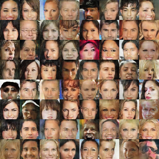
Figure 6-15. Images sampled from a generative adversarial network (GAN) trained on a dataset of faces. Note that sampled images are less blurry than those from the variational autoencoder.

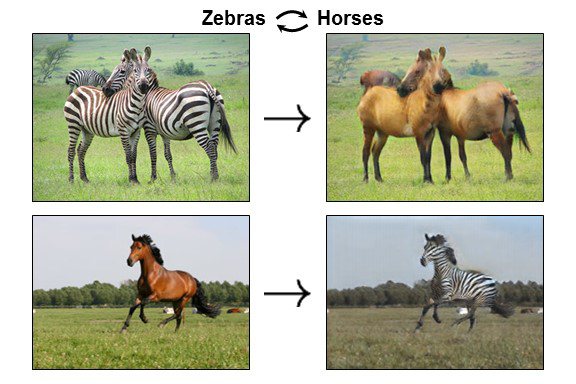
Figure 6-16. The CycleGAN is capable of performing complex image transformations, such as transforming images of horses into those of zebras (and vice versa).

Unfortunately, generative adversarial networks are still challenging to train in practice. Making generators and discriminators learn reasonable functions requires a deep bag of tricks. As a result, while there have been many exciting GAN demonstrations, GANs have not yet matured into a state where they can be widely deployed in industrial applications.

The MNIST Dataset

The MNIST dataset consists of images of handwritten digits. The machine learning challenge associated with MNIST consists of creating a model trained on the training set of digits that generalizes to the validation set. Figure 6-17 shows some images drawn from the MNIST dataset.

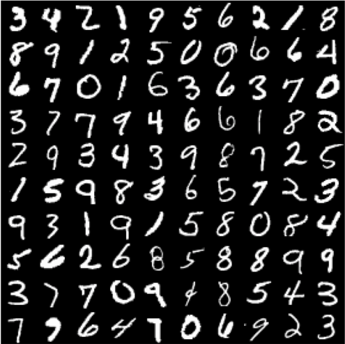
Figure 6-17. Some images of handwritten digits from the MNIST dataset. The learning challenge is to predict the digit from the image.

MNIST was a very important dataset for the development of machine learning methods for computer vision. The dataset is challenging enough that obvious, non-learning methods don’t tend to do well. At the same time, MNIST is small enough that experimenting with new architectures doesn’t require very large amounts of computing power.

However, the MNIST dataset has mostly become obsolete. The best models achieve near one hundred percent test accuracy. Note that this fact doesn’t mean that the problem of handwritten digit recognition is solved! Rather, it is likely that human scientists have overfit architectures to the MNIST dataset and capitalized on its quirks to achieve very high predictive accuracies. As a result, it’s no longer good practice to use MNIST to design new deep architectures. That said, MNIST is still a superb dataset for pedagogical purposes.

Loading MNIST

The MNIST codebase is located online on Yann LeCun’s website. The download script pulls down the raw file from the website. Notice how the script caches the download so repeated calls to download() won’t waste effort.

As a more general note, it’s quite common to store ML datasets in the cloud and have user code retrieve it before processing for input into a learning algorithm. The Tox21 dataset we accessed via the DeepChem library in Chapter 4 followed this same design pattern. In general, if you would like to host a large dataset for analysis, hosting on the cloud and downloading to a local machine for processing as necessary seems good practice. (This breaks down for very large datasets however, where network transfer times become exorbitantly expensive.) See Example 6-1.

def download(filename):
  """Download the data from Yann's website, unless it's already here."""
  if not os.path.exists(WORK_DIRECTORY):
    os.makedirs(WORK_DIRECTORY)
  filepath = os.path.join(WORK_DIRECTORY, filename)
  if not os.path.exists(filepath):
    filepath, _ = urllib.request.urlretrieve(SOURCE_URL + filename, filepath)
    size = os.stat(filepath).st_size
    print('Successfully downloaded', filename, size, 'bytes.')
  return filepath

This download checks for the existence of WORK_DIRECTORY. If this directory exists, it assumes that the MNIST dataset has already been downloaded. Else, the script uses the urllib Python library to perform the download and prints the number of bytes downloaded.

The MNIST dataset is stored as a raw string of bytes encoding pixel values. In order to easily process this data, we need to convert it into a NumPy array. The function np.frombuffer provides a convenience that allows the conversion of a raw byte buffer into a numerical array (Example 6-2). As we have noted elsewhere in this book, deep networks can be destabilized by input data that occupies wide ranges. For stable gradient descent, it is often necessary to constrain inputs to span a bounded range. The original MNIST dataset contains pixel values ranging from 0 to 255. For stability, this range needs to be shifted to have mean zero and unit range (from –0.5 to +0.5).

def extract_data(filename, num_images):
  """Extract the images into a 4D tensor [image index, y, x, channels].

  Values are rescaled from [0, 255] down to [-0.5, 0.5].
  """
  print('Extracting', filename)
  with gzip.open(filename) as bytestream:
    bytestream.read(16)
    buf = bytestream.read(IMAGE_SIZE * IMAGE_SIZE * num_images * NUM_CHANNELS)
    data = numpy.frombuffer(buf, dtype=numpy.uint8).astype(numpy.float32)
    data = (data - (PIXEL_DEPTH / 2.0)) / PIXEL_DEPTH
    data = data.reshape(num_images, IMAGE_SIZE, IMAGE_SIZE, NUM_CHANNELS)
    return data

The labels are stored in a simple file as a string of bytes. There is a header consisting of 8 bytes, with the remainder of the data containing labels (Example 6-3).

def extract_labels(filename, num_images):
  """Extract the labels into a vector of int64 label IDs."""
  print('Extracting', filename)
  with gzip.open(filename) as bytestream:
    bytestream.read(8)
    buf = bytestream.read(1 * num_images)
    labels = numpy.frombuffer(buf, dtype=numpy.uint8).astype(numpy.int64)
  return labels

Given the functions defined in the previous examples, it is now feasible to download and process the MNIST training and test dataset (Example 6-4).

# Get the data.
train_data_filename = download('train-images-idx3-ubyte.gz')
train_labels_filename = download('train-labels-idx1-ubyte.gz')
test_data_filename = download('t10k-images-idx3-ubyte.gz')
test_labels_filename = download('t10k-labels-idx1-ubyte.gz')

# Extract it into NumPy arrays.
train_data = extract_data(train_data_filename, 60000)
train_labels = extract_labels(train_labels_filename, 60000)
test_data = extract_data(test_data_filename, 10000)
test_labels = extract_labels(test_labels_filename, 10000)

The MNIST dataset doesn’t explicitly define a validation dataset for hyperparameter tuning. Consequently, we manually designate the final 5,000 datapoints of the training dataset as validation data (Example 6-5).

VALIDATION_SIZE = 5000  # Size of the validation set.

# Generate a validation set.
validation_data = train_data[:VALIDATION_SIZE, ...]
validation_labels = train_labels[:VALIDATION_SIZE]
train_data = train_data[VALIDATION_SIZE:, ...]
train_labels = train_labels[VALIDATION_SIZE:]

TensorFlow Convolutional Primitives

We start by introducing the TensorFlow primitives that are used to construct our convolutional networks (Example 6-6).

tf.nn.conv2d(
    input,
    filter,
    strides,
    padding,
    use_cudnn_on_gpu=None,
    data_format=None,
    name=None
)

The function tf.nn.conv2d is the built-in TensorFlow function that defines convolutional layers. Here, input is assumed to be a tensor of shape (batch, height, width, channels) where batch is the number of images in a minibatch.

Note that the conversion functions defined previously read the MNIST data into this format. The argument filter is a tensor of shape (filter_height, filter_width, channels, out_channels) that specifies the learnable weights for the nonlinear transformation learned in the convolutional kernel. strides contains the filter strides and is a list of length 4 (one for each input dimension).

padding controls whether the input tensors are padded (with extra zeros as in Figure 6-18) to guarantee that output from the convolutional layer has the same shape as the input. If padding="SAME", then input is padded to ensure that the convolutional layer outputs an image tensor of the same shape as the original input image tensor. If padding="VALID" then extra padding is not added.

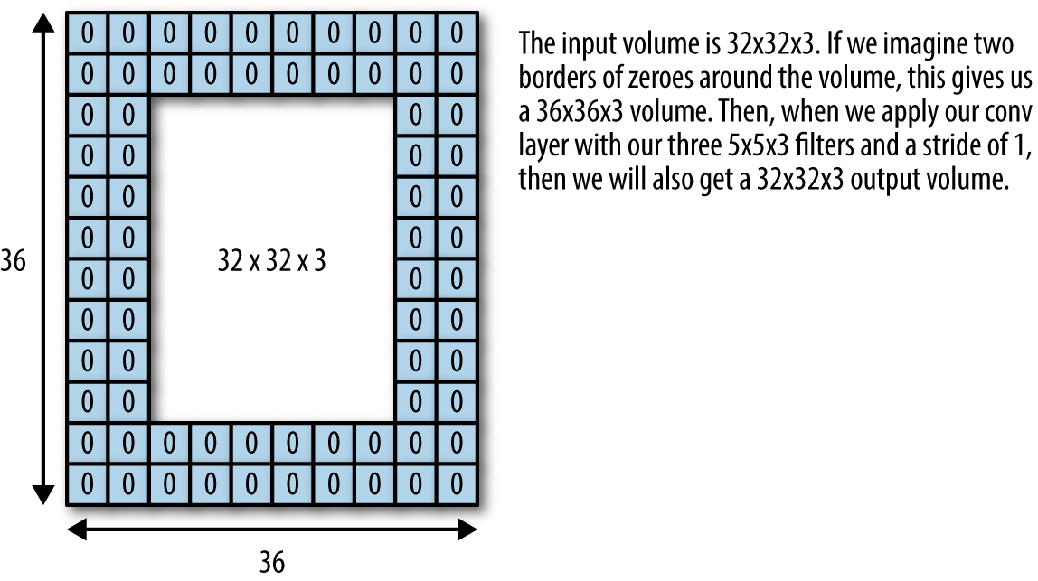
Figure 6-18. Padding for convolutional layers ensures that the output image has the same shape as the input image.

The code in Example 6-7 defines max pooling in TensorFlow.

tf.nn.max_pool(
    value,
    ksize,
    strides,
    padding,
    data_format='NHWC',
    name=None
)

The tf.nn.max_pool function performs max pooling. Here value has the same shape as input for tf.nn.conv2d, (batch, height, width, channels). ksize is the size of the pooling window and is a list of length 4. strides and padding behave as for tf.nn.conv2d.

The Convolutional Architecture

The architecture defined in this section will closely resemble LeNet-5, the original architecture used to train convolutional neural networks on the MNIST dataset. At the time the LeNet-5 architecture was invented, it was exorbitantly expensive computationally, requiring multiple weeks of compute to complete training. Today’s laptops thankfully are more than sufficient to train LeNet-5 models. Figure 6-19 illustrates the structure of the LeNet-5 architecture.

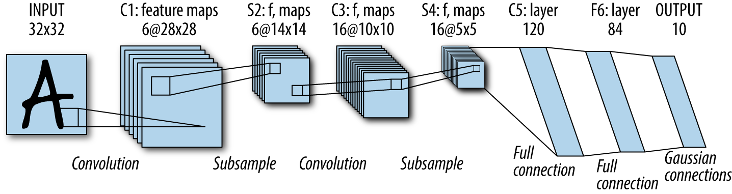
Figure 6-19. An illustration of the LeNet-5 convolutional architecture.

Let’s define the weights needed to train our LeNet-5 network. We start by defining some basic constants that are used to define our weight tensors (Example 6-8).

NUM_CHANNELS = 1
IMAGE_SIZE = 28
NUM_LABELS = 10

The architecture we define will use two convolutional layers interspersed with two pooling layers, topped off by two fully connected layers. Recall that pooling requires no learnable weights, so we simply need to create weights for the convolutional and fully connected layers. For each tf.nn.conv2d, we need to create a learnable weight tensor corresponding to the filter argument for tf.nn.conv2d. In this particular architecture, we will also add a convolutional bias, one for each output channel (Example 6-9).

conv1_weights = tf.Variable(
    tf.truncated_normal([5, 5, NUM_CHANNELS, 32],  # 5x5 filter, depth 32.
                        stddev=0.1,
                        seed=SEED, dtype=tf.float32))
conv1_biases = tf.Variable(tf.zeros([32], dtype=tf.float32))
conv2_weights = tf.Variable(tf.truncated_normal(
    [5, 5, 32, 64], stddev=0.1,
    seed=SEED, dtype=tf.float32))
conv2_biases = tf.Variable(tf.constant(0.1, shape=[64], dtype=tf.float32))

Note that the convolutional weights are 4-tensors, while the biases are 1-tensors. The first fully connected layer converts the outputs of the convolutional layer to a vector of size 512. The input images start with size IMAGE_SIZE=28. After the two pooling layers (each of which reduces the input by a factor of 2), we end with images of size IMAGE_SIZE//4. We create the shape of the fully connected weights accordingly.

The second fully connected layer is used to provide the 10-way classification output, so it has weight shape (512,10) and bias shape (10), shown in Example 6-10.

fc1_weights = tf.Variable(  # fully connected, depth 512.
    tf.truncated_normal([IMAGE_SIZE // 4 * IMAGE_SIZE // 4 * 64, 512],
                        stddev=0.1,
                        seed=SEED,
                        dtype=tf.float32))
fc1_biases = tf.Variable(tf.constant(0.1, shape=[512], dtype=tf.float32))
fc2_weights = tf.Variable(tf.truncated_normal([512, NUM_LABELS],
                                              stddev=0.1,
                                              seed=SEED,
                                              dtype=tf.float32))
fc2_biases = tf.Variable(tf.constant(
    0.1, shape=[NUM_LABELS], dtype=tf.float32))

With all the weights defined, we are now free to define the architecture of the network. The architecture has six layers in the pattern conv-pool-conv-pool-full-full (Example 6-11).

def model(data, train=False):
  """The Model definition."""
  # 2D convolution, with 'SAME' padding (i.e. the output feature map has
  # the same size as the input). Note that {strides} is a 4D array whose
  # shape matches the data layout: [image index, y, x, depth].
  conv = tf.nn.conv2d(data,
                      conv1_weights,
                      strides=[1, 1, 1, 1],
                      padding='SAME')
  # Bias and rectified linear non-linearity.
  relu = tf.nn.relu(tf.nn.bias_add(conv, conv1_biases))
  # Max pooling. The kernel size spec {ksize} also follows the layout of
  # the data. Here we have a pooling window of 2, and a stride of 2.
  pool = tf.nn.max_pool(relu,
                        ksize=[1, 2, 2, 1],
                        strides=[1, 2, 2, 1],
                        padding='SAME')
  conv = tf.nn.conv2d(pool,
                      conv2_weights,
                      strides=[1, 1, 1, 1],
                      padding='SAME')
  relu = tf.nn.relu(tf.nn.bias_add(conv, conv2_biases))
  pool = tf.nn.max_pool(relu,
                        ksize=[1, 2, 2, 1],
                        strides=[1, 2, 2, 1],
                        padding='SAME')
  # Reshape the feature map cuboid into a 2D matrix to feed it to the
  # fully connected layers.
  pool_shape = pool.get_shape().as_list()
  reshape = tf.reshape(
      pool,
      [pool_shape[0], pool_shape[1] * pool_shape[2] * pool_shape[3]])
  # Fully connected layer. Note that the '+' operation automatically
  # broadcasts the biases.
  hidden = tf.nn.relu(tf.matmul(reshape, fc1_weights) + fc1_biases)
  # Add a 50% dropout during training only. Dropout also scales
  # activations such that no rescaling is needed at evaluation time.
  if train:
    hidden = tf.nn.dropout(hidden, 0.5, seed=SEED)
  return tf.matmul(hidden, fc2_weights) + fc2_biases

As noted previously, the basic architecture of the network intersperses tf.nn.conv2d, tf.nn.max_pool, with nonlinearities, and a final fully connected layer. For regularization, a dropout layer is applied after the final fully connected layer, but only during training. Note that we pass in the input as an argument data to the function model().

The only part of the network that remains to be defined are the placeholders (Example 6-12). We need to define two placeholders for inputting the training images and the training labels. In this particular network, we also define a separate placeholder for evaluation that allows us to input larger batches when evaluating.

BATCH_SIZE = 64
EVAL_BATCH_SIZE = 64

train_data_node = tf.placeholder(
    tf.float32,
    shape=(BATCH_SIZE, IMAGE_SIZE, IMAGE_SIZE, NUM_CHANNELS))
train_labels_node = tf.placeholder(tf.int64, shape=(BATCH_SIZE,))
eval_data = tf.placeholder(
    tf.float32,
    shape=(EVAL_BATCH_SIZE, IMAGE_SIZE, IMAGE_SIZE, NUM_CHANNELS))

With these definitions in place, we now have the data processed, inputs and weights specified, and the model constructed. We are now prepared to train the network (Example 6-13).

# Create a local session to run the training.
start_time = time.time()
with tf.Session() as sess:
  # Run all the initializers to prepare the trainable parameters.
  tf.global_variables_initializer().run()
  # Loop through training steps.
  for step in xrange(int(num_epochs * train_size) // BATCH_SIZE):
    # Compute the offset of the current minibatch in the data.
    # Note that we could use better randomization across epochs.
    offset = (step * BATCH_SIZE) % (train_size - BATCH_SIZE)
    batch_data = train_data[offset:(offset + BATCH_SIZE), ...]
    batch_labels = train_labels[offset:(offset + BATCH_SIZE)]
    # This dictionary maps the batch data (as a NumPy array) to the
    # node in the graph it should be fed to.
    feed_dict = {train_data_node: batch_data,
                 train_labels_node: batch_labels}
    # Run the optimizer to update weights.
    sess.run(optimizer, feed_dict=feed_dict)

The structure of this fitting code looks quite similar to other code for fitting we’ve seen so far in this book. In each step, we construct a feed dictionary, and then run a step of the optimizer. Note that we use minibatch training as before.

Evaluating Trained Models

We now have a model training. How can we evaluate the accuracy of the trained model? A simple method is to define an error metric. As in previous chapters, we shall use a simple classification metric to gauge accuracy (Example 6-14).

def error_rate(predictions, labels):
  """Return the error rate based on dense predictions and sparse labels."""
  return 100.0 - (
      100.0 *
      numpy.sum(numpy.argmax(predictions, 1) == labels) /
      predictions.shape[0])

We can use this function to evaluate the error of the network as we train. Let’s introduce an additional convenience function that evaluates predictions on any given dataset in batches (Example 6-15). This convenience is necessary since our network can only handle inputs with fixed batch sizes.

def eval_in_batches(data, sess):
  """Get predictions for a dataset by running it in small batches."""
  size = data.shape[0]
  if size < EVAL_BATCH_SIZE:
    raise ValueError("batch size for evals larger than dataset: %d"
                     % size)
  predictions = numpy.ndarray(shape=(size, NUM_LABELS),
                              dtype=numpy.float32)
  for begin in xrange(0, size, EVAL_BATCH_SIZE):
    end = begin + EVAL_BATCH_SIZE
    if end <= size:
      predictions[begin:end, :] = sess.run(
          eval_prediction,
          feed_dict={eval_data: data[begin:end, ...]})
    else:
      batch_predictions = sess.run(
          eval_prediction,
          feed_dict={eval_data: data[-EVAL_BATCH_SIZE:, ...]})
      predictions[begin:, :] = batch_predictions[begin - size:, :]
  return predictions

We can now add a little instrumentation (in the inner for-loop of training) that periodically evaluates the model’s accuracy on the validation set. We can end training by scoring test accuracy. Example 6-16 shows the full fitting code with instrumentation added in.

# Create a local session to run the training.
start_time = time.time()
with tf.Session() as sess:
  # Run all the initializers to prepare the trainable parameters.
  tf.global_variables_initializer().run()
  # Loop through training steps.
  for step in xrange(int(num_epochs * train_size) // BATCH_SIZE):
    # Compute the offset of the current minibatch in the data.
    # Note that we could use better randomization across epochs.
    offset = (step * BATCH_SIZE) % (train_size - BATCH_SIZE)
    batch_data = train_data[offset:(offset + BATCH_SIZE), ...]
    batch_labels = train_labels[offset:(offset + BATCH_SIZE)]
    # This dictionary maps the batch data (as a NumPy array) to the
    # node in the graph it should be fed to.
    feed_dict = {train_data_node: batch_data,
                 train_labels_node: batch_labels}
    # Run the optimizer to update weights.
    sess.run(optimizer, feed_dict=feed_dict)
    # print some extra information once reach the evaluation frequency
    if step % EVAL_FREQUENCY == 0:
      # fetch some extra nodes' data
      l, lr, predictions = sess.run([loss, learning_rate,
                                     train_prediction],
                                    feed_dict=feed_dict)
      elapsed_time = time.time() - start_time
      start_time = time.time()
      print('Step %d (epoch %.2f), %.1f ms' %
            (step, float(step) * BATCH_SIZE / train_size,
             1000 * elapsed_time / EVAL_FREQUENCY))
      print('Minibatch loss: %.3f, learning rate: %.6f' % (l, lr))
      print('Minibatch error: %.1f%%'
            % error_rate(predictions, batch_labels))
      print('Validation error: %.1f%%' % error_rate(
          eval_in_batches(validation_data, sess), validation_labels))
      sys.stdout.flush()
  # Finally print the result!
  test_error = error_rate(eval_in_batches(test_data, sess),
                          test_labels)
  print('Test error: %.1f%%' % test_error)

Challenge for the Reader

Try training the network yourself. You should be able to achieve test error of < 1%!