Chapter 9. Training Large Deep Networks
Thus far, you have seen how to train small models that can be completely trained on a good laptop computer. All of these models can be run fruitfully on GPU-equipped hardware with notable speed boosts (with the notable exception of reinforcement learning models for reasons discussed in the previous chapter). However, training larger models still requires considerable sophistication. In this chapter, we will discuss various types of hardware that can be used to train deep networks, including graphics processing units (GPUs), tensor processing units (TPUs), and neuromorphic chips. We will also briefly cover the principles of distributed training for larger deep learning models. We end the chapter with an in-depth case study, adapated from one of the TensorFlow tutorials, demonstrating how to train a CIFAR-10 convolutional neural network on a server with multiple GPUs. We recommend that you attempt to try running this code yourself, but readily acknowledge that gaining access to a multi-GPU server is trickier than finding a good laptop. Luckily, access to multi-GPU servers on the cloud is becoming possible and is likely the best solution for industrial users of TensorFlow seeking to train large models.
Custom Hardware for Deep Networks
As you’ve seen throughout the book, deep network training requires chains of tensorial operations performed repeatedly on minibatches of data. Tensorial operations are commonly transformed into matrix multiplication operations by software, so rapid training of deep networks fundamentally depends on the ability to perform matrix multiplication operations rapidly. While CPUs are perfectly capable of implementing matrix multiplications, the generality of CPU hardware means much effort will be wasted on overhead unneeded for mathematical operations.
Hardware engineers have noted this fact for years, and there exist a variety of alternative hardware for working with deep networks. Such hardware can be broadly divided into inference only or training and inference. Inference-only hardware cannot be used to train new deep networks, but can be used to deploy trained models in production, allowing for potentially orders-of-magnitude increases in performance. Training and inference hardware allows for models to be trained natively. Currently, Nvidia’s GPU hardware holds a dominant position in the training and inference market due to significant investment in software and outreach by Nvidia’s teams, but a number of other competitors are snapping at the GPU’s heels. In this section, we will briefly cover some of these newer hardware alternatives. With the exception of GPUs and CPUs, most of these alternative forms of hardware are not yet widely available, so much of this section is forward looking.
CPU Training
Although CPU training is by no means state of the art for training deep networks, it often does quite well for smaller models (as you’ve seen firsthand in this book). For reinforcement learning problems, a multicore CPU machine can even outperform GPU training.
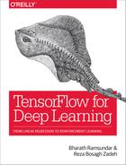
CPUs also see wide usage for inference-only applications of deep networks. Most companies have invested heavily in developing cloud servers built primarily on Intel server boxes. It’s very likely that the first generation of deep networks deployed widely (outside tech companies) will be primarily deployed into production on such Intel servers. While such CPU-based deployment isn’t sufficient for heavy-duty deployment of learning models, it is often plenty for first customer needs. Figure 9-1 illustrates a standard Intel CPU.
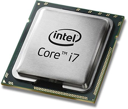
Figure 9-1. A CPU from Intel. CPUs are still the dominant form of computer hardware and are present in all modern laptops, desktops, servers, and phones. Most software is written to execute on CPUs. Numerical computations (such as neural network training) can be executed on CPUs, but might be slower than on customized hardware optimized for numerical methods.
GPU Training
GPUs were first developed to perform computations needed by the graphics community. In a fortuitous coincidence, it turned out that the primitives used to define graphics shaders could be repurposed to perform deep learning. At their mathematical hearts, both graphics and machine learning rely critically on matrix multiplications. Empirically, GPU matrix multiplications offer speedups of an order of magnitude or two over CPU implementations. How do GPUs succeed at this feat? The trick is that GPUs make use of thousands of identical threads. Clever hackers have succeeded in decomposing matrix multiplications into massively parallel operations that can offer dramatic speedups. Figure 9-2 illustrates a GPU architecture.
Although there are a number of GPU vendors, Nvidia currently dominates the GPU market. Much of the power of Nvidia’s GPUs stems from its custom library CUDA (compute unified device architecture), which offers primitives that make it easier to write GPU programs. Nvidia offers a CUDA extension, CUDNN, for speeding up deep networks (Figure 9-2). TensorFlow has built-in CUDNN support, so you can make use of CUDNN to speed up your networks as well through TensorFlow.
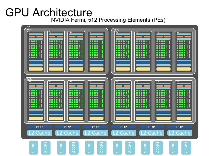
Figure 9-2. A GPU architecture from Nvidia. GPUs possess many more cores than CPUs and are well suited to performing numerical linear algebra, of the sort useful in both graphics and machine learning computations. GPUs have emerged as the dominant hardware platform for training deep networks.
How Important Are Transistor Sizes?
For years, the semiconductor industry has tracked progression of chip speeds by watching transistor sizes. As transistors got smaller, more of them could be packed onto a standard chip, and algorithms could run faster. At the time of writing of this book, Intel is currently operating on 10-nanometer transistors, and working on transitioning down to 7 nanometers. The rate of shrinkage of transistor sizes has slowed significantly in recent years, since formidable heat dissipation issues arise at these scales.
Nvidia’s GPUs partially buck this trend. They tend to use transistor sizes a generation or two behind Intel’s best, and focus on solving architectural and software bottlenecks instead of transistor engineering. So far, Nvidia’s strategy has paid dividends and the company has achieved market domination in the machine learning chip space.
It’s not yet clear how far architectural and software optimizations can go. Will GPU optimizations soon run into the same Moore’s law roadblocks as CPUs? Or will clever architectural innovations enable years of faster GPUs? Only time can tell.
Tensor Processing Units
The tensor processing unit (TPU) is a custom ASIC (application specific integrated circuit) designed by Google to speed up deep learning workloads designed in TensorFlow. Unlike the GPU, the TPU is stripped down and implements only the bare minimum on-die needed to perform necessary matrix multiplications. Unlike the GPU, the TPU is dependent on an adjoining CPU to do much of its preprocessing work for it. This slimmed-down approach enables the TPU to achieve higher speeds than the GPU at lower energy costs.
The first version of the TPU only allowed for inference on trained models, but the most recent version (TPU2) allows for training of (certain) deep networks as well. However, Google has not released many details about the TPU, and access is limited to Google collaborators, with plans to enable TPU access via the Google cloud. Nvidia is taking notes from the TPU, and it’s quite likely that future releases of Nvidia GPUs will come to resemble the TPU, so downstream users will likely benefit from Google’s innovations regardless of whether Google or Nvidia wins the consumer deep learning market. Figure 9-3 illustrates the TPU architecture design.
Figure 9-3. A tensor processing unit (TPU) architecture from Google. TPUs are specialized chips designed by Google to speed up deep learning workloads. The TPU is a coprocessor and not a standalone piece of hardware.
What Are ASICs?
Both CPUs and GPUs are general-purpose chips. CPUs generally support instruction sets in assembly and are designed to be universal. Care is taken to enable a wide range of applications. GPUs are less universal, but still allow for a wide range of algorithms to be implemented via languages such as CUDA.
Application specific integrated circuits (ASICs) attempt to do away with the generality in favor of focusing on the needs of a particular application. Historically, ASICs have only achieved limited market penetration. The drumbeat of Moore’s law meant that general-purpose CPUs stayed only a breath or two behind custom ASICs, so the hardware design overhead was often not worth the effort.
This state of affairs has started shifting in the last few years. The slowdown of transistor shrinkage has expanded ASIC usage. For example, Bitcoin mining depends entirely on custom ASICs that implement specialized cryptography operations.
Field Programmable Gate Arrays
Field programmable gate arrays (FPGAs) are a type of “field programmable” ASIC. Standard FPGAs can often be reconfigured via hardware description languages such as Verilog to implement new ASIC designs dynamically. While FPGAs are generally less efficient than custom ASICs, they can offer significant speed improvements over CPU implementations. Microsoft in particular has used FPGAs to perform deep learning inference and claims to have achieved significant speedups with their deployment. However, the approach has not yet caught on widely outside Microsoft.
Neuromorphic Chips
The “neurons” in deep networks mathematically model the 1940s understanding of neuronal biology. Needless to say, biological understanding of neuronal behavior has progressed dramatically since then. For one, it’s now known that the nonlinear activations used in deep networks aren’t accurate models of neuronal nonlinearity. The “spike trains” is a better model (see Figure 9-4), where neurons activate in short-lived bursts (spikes) but fall to background most of the time.
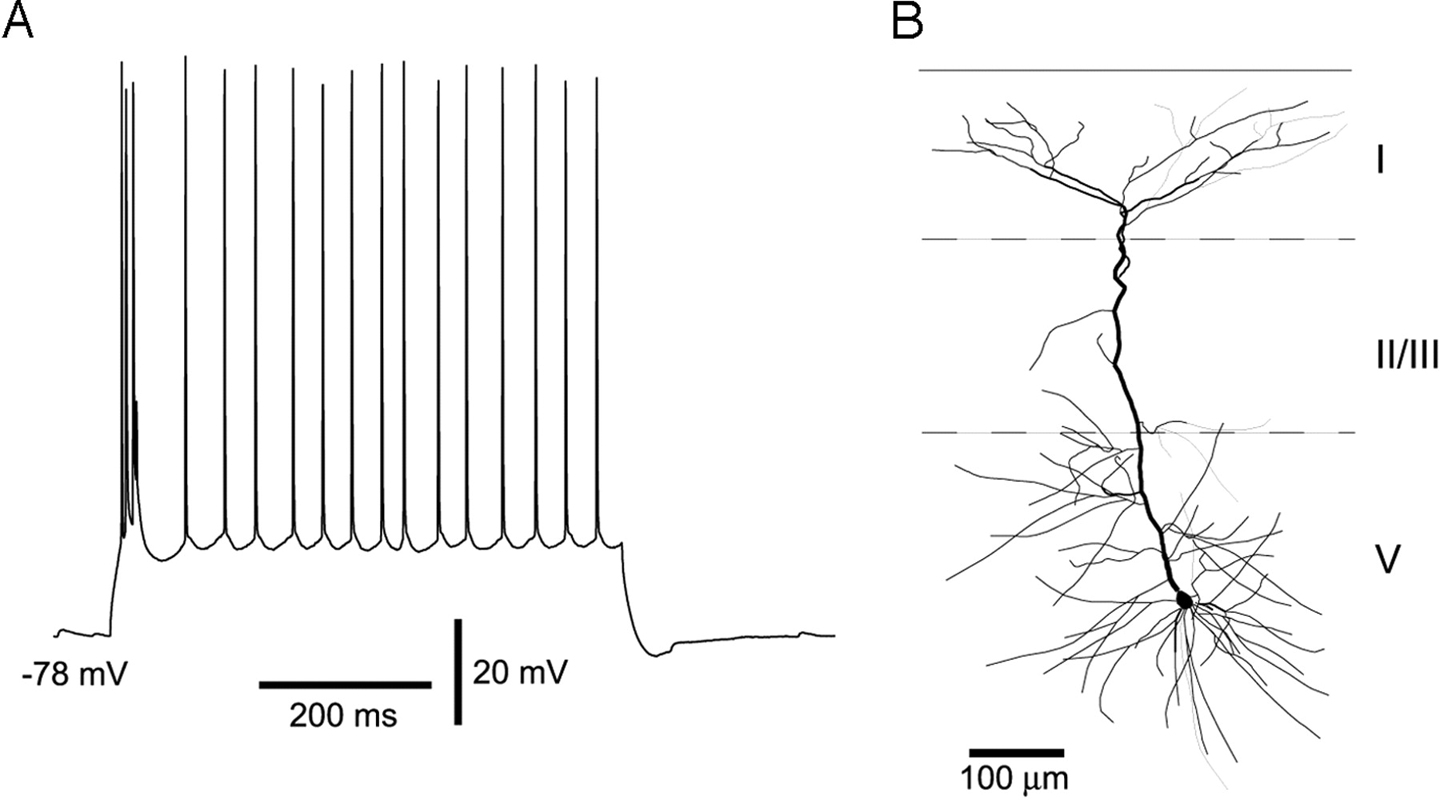
Figure 9-4. Neurons often activate in short-lived bursts called spike trains (A). Neuromorphic chips attempt to model spiking behavior in computing hardware. Biological neurons are complex entities (B), so these models are still only approximate.
Hardware engineers have spent significant effort exploring whether it’s possible to create chip designs based on spike trains rather than on existing circuit technologies (CPUs, GPUs, ASICs). These designers argue that today’s chip designs suffer from fundamental power limitations; the brain consumes many orders of magnitude less power than computer chips and smart designs should aim to learn from the brain’s architecture.
A number of projects have built large spike train chips attempting to expand upon this core thesis. IBM’s TrueNorth project has succeeded in building spike train processors with millions of “neurons” and demonstrated that this hardware can perform basic image recognition with significantly lower power requirements than existing chip designs. However, despite these successes, it is not clear how to translate modern deep architectures onto spike train chips. Without the ability to “compile” TensorFlow models onto spike train hardware, it’s unlikely that such projects will see widespread adoption in the near future.
Distributed Deep Network Training
In the previous section, we surveyed a variety of hardware options for training deep networks. However, most organizations will likely only have access to CPUs and perhaps GPUs. Luckily, it’s possible to perform distributed training of deep networks, where multiple CPUs or GPUs are used to train models faster and more effectively. Figure 9-5 illustrates the two major paradigms for training deep networks with multiple CPUs/GPUs, namely data parallel and model parallel training. You will learn about these methods in more detail in the next two sections.
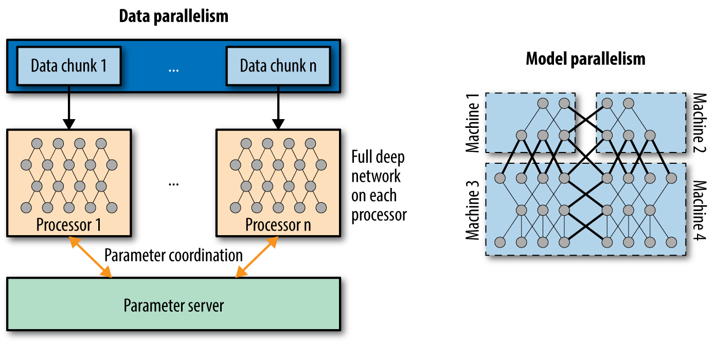
Figure 9-5. Data parallelism and model parallelism are the two main modes of distributed training of deep architectures. Data parallel training splits large datasets across multiple computing nodes, while model parallel training splits large models across multiple nodes. The next two sections will cover these two methods in greater depth.
Data Parallelism
Data parallelism is the most common type of multinode deep network training. Data parallel models split large datasets onto different machines. Most nodes are workers and have access to a fraction of the total data used to train the network. Each worker node has a complete copy of the model being trained. One node is designated as the supervisor that gathers updated weights from the workers at regular intervals and pushes averaged versions of the weights out to worker nodes. Note that you’ve already seen a data parallel example in this book; the A3C implementation presented in Chapter 8 is a simple example of data parallel deep network training.
As a historical note, Google’s predecessor to TensorFlow, DistBelief, was based on data parallel training on CPU servers. This system was capable of achieving distributed CPU speeds (using 32–128 nodes) that matched or exceeded GPU training speeds. Figure 9-6 illustrates the data parallel training method implemented by DistBelief. However, the success of systems like DistBelief tends to depend on the presence of high throughput network interconnects that can allow for rapid model parameter sharing. Many organizations lack the network infrastructure that enables effective multinode data parallel CPU training. However, as the A3C example demonstrates, it is possible to perform data parallel training on a single node, using different CPU cores. For modern servers, it is also possible to perform data parallel training using multiple GPUs stocked within a single server, as we will show you later.
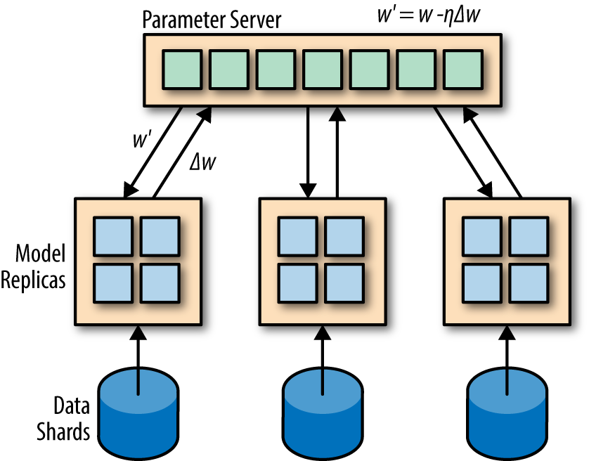
Figure 9-6. The Downpour stochastic gradient descent (SGD) method maintains multiple replicas of the model and trains them on different subsets of a dataset. The learned weights from these shards are periodically synced to global weights stored on a parameter server.
Model Parallelism
The human brain provides the only known example of a generally intelligent piece of hardware, so there have naturally been comparisons drawn between the complexity of deep networks and the complexity of the brain. Simple arguments state the brain has roughly 100 billion neurons; would constructing deep networks with that many “neurons” suffice to achieve general intelligence? Unfortunately, such arguments miss the point that biological neurons are significantly more complex than “mathematical neurons.” As a result, simple comparisons yield little value. Nonetheless, building larger deep networks has been a major research focus over the last few years.
The major difficulty with training very large deep networks is that GPUs tend to have limited memory (dozens of gigabytes typically). Even with careful encodings, neural networks with more than a few hundred million parameters are not feasible to train on single GPUs due to memory requirements. Model parallel training algorithms attempt to sidestep this limitation by storing large deep networks on the memories of multiple GPUs. A few teams have successfully implemented these ideas on arrays of GPUs to train deep networks with billions of parameters. Unfortunately, these models have not thus far shown performance improvements justifying the extra difficulty. For now, it seems that the increase in experimental ease from using smaller models outweighs the gains from model parallelism.
Hardware Memory Interconnects
Enabling model parallelism requires having very high bandwidth connections between compute nodes since each gradient update by necessity requires internode communication. Note that while data parallelism requires strong interconnects, sync operations need only be performed sporadically after multiple local gradient updates.
A few groups have used InfiniBand interconnects (InfiniBand is a high-throughput, low-latency networking standard), or Nvidia’s proprietary NVLINK interconnects to attempt to build such large models. However, the results from such experiments have been mixed thus far, and the hardware requirements for such systems tend to be expensive.
Data Parallel Training with Multiple GPUs on Cifar10
In this section, we will give you an in-depth walkthrough of how to train a data-parallel convolutional network on the Cifar10 benchmark set. Cifar10 consists of 60,000 images of size 32 × 32. The Cifar10 dataset is often used to benchmark convolutional architectures. Figure 9-7 displays sample images from the Cifar10 dataset.
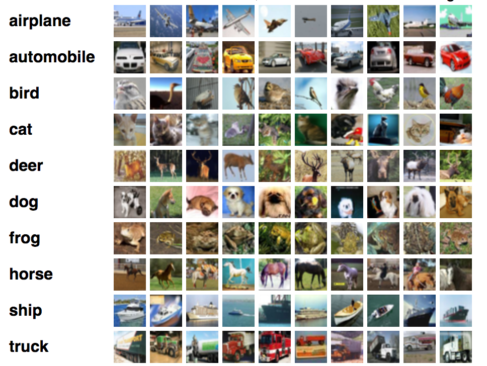
Figure 9-7. The Cifar10 dataset consists of 60,000 images drawn from 10 classes. Some sample images from various classes are displayed here.
The architecture we will use in this section loads separate copies of the model architecture on different GPUs and periodically syncs learned weights across cores, as Figure 9-8 illustrates.
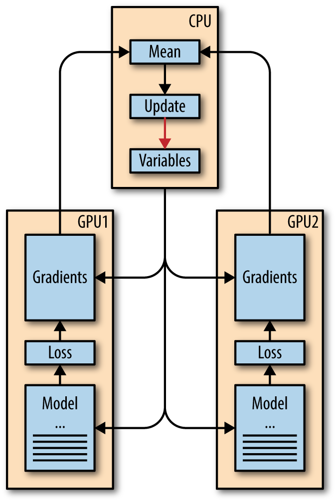
Figure 9-8. The data parallel architecture you will train in this chapter.
Downloading and Loading the DATA
The read_cifar10() method reads and parses the Cifar10 raw data files. Example 9-1 uses tf.FixedLengthRecordReader to read raw data from the Cifar10 files.
Example 9-1. This function reads and parses data from Cifar10 raw data files
defread_cifar10(filename_queue):"""Reads and parses examples from CIFAR10 data files.Recommendation: if you want N-way read parallelism, call this functionN times. This will give you N independent Readers reading differentfiles & positions within those files, which will give better mixing ofexamples.Args:filename_queue: A queue of strings with the filenames to read from.Returns:An object representing a single example, with the following fields:height: number of rows in the result (32)width: number of columns in the result (32)depth: number of color channels in the result (3)key: a scalar string Tensor describing the filename & record numberfor this example.label: an int32 Tensor with the label in the range 0..9.uint8image:: a [height, width, depth] uint8 Tensor with the image data"""classCIFAR10Record(object):passresult=CIFAR10Record()# Dimensions of the images in the CIFAR-10 dataset.# See http://www.cs.toronto.edu/~kriz/cifar.html for a description of the# input format.label_bytes=1# 2 for CIFAR-100result.height=32result.width=32result.depth=3image_bytes=result.height*result.width*result.depth# Every record consists of a label followed by the image, with a# fixed number of bytes for each.record_bytes=label_bytes+image_bytes# Read a record, getting filenames from the filename_queue. No# header or footer in the CIFAR-10 format, so we leave header_bytes# and footer_bytes at their default of 0.reader=tf.FixedLengthRecordReader(record_bytes=record_bytes)result.key,value=reader.read(filename_queue)# Convert from a string to a vector of uint8 that is record_bytes long.record_bytes=tf.decode_raw(value,tf.uint8)# Read a record, getting filenames from the filename_queue. No# header or footer in the CIFAR-10 format, so we leave header_bytes# and footer_bytes at their default of 0.reader=tf.FixedLengthRecordReader(record_bytes=record_bytes)result.key,value=reader.read(filename_queue)# Convert from a string to a vector of uint8 that is record_bytes long.record_bytes=tf.decode_raw(value,tf.uint8)# The first bytes represent the label, which we convert from uint8->int32.result.label=tf.cast(tf.strided_slice(record_bytes,[0],[label_bytes]),tf.int32)# The remaining bytes after the label represent the image, which we reshape# from [depth * height * width] to [depth, height, width].depth_major=tf.reshape(tf.strided_slice(record_bytes,[label_bytes],[label_bytes+image_bytes]),[result.depth,result.height,result.width])# Convert from [depth, height, width] to [height, width, depth].result.uint8image=tf.transpose(depth_major,[1,2,0])returnresult
Deep Dive on the Architecture
The architecture for the network is a standard multilayer convnet, similar to a more complicated version of the LeNet5 architecture you saw in Chapter 6. The inference() method constructs the architecture (Example 9-2). This convolutional architecture follows a relatively standard architecture, with convolutional layers interspersed with local normalization layers.
Example 9-2. This function builds the Cifar10 architecture
definference(images):"""Build the CIFAR10 model.Args:images: Images returned from distorted_inputs() or inputs().Returns:Logits."""# We instantiate all variables using tf.get_variable() instead of# tf.Variable() in order to share variables across multiple GPU training runs.# If we only ran this model on a single GPU, we could simplify this function# by replacing all instances of tf.get_variable() with tf.Variable().## conv1withtf.variable_scope('conv1')asscope:kernel=_variable_with_weight_decay('weights',shape=[5,5,3,64],stddev=5e-2,wd=0.0)conv=tf.nn.conv2d(images,kernel,[1,1,1,1],padding='SAME')biases=_variable_on_cpu('biases',[64],tf.constant_initializer(0.0))pre_activation=tf.nn.bias_add(conv,biases)conv1=tf.nn.relu(pre_activation,name=scope.name)_activation_summary(conv1)# pool1pool1=tf.nn.max_pool(conv1,ksize=[1,3,3,1],strides=[1,2,2,1],padding='SAME',name='pool1')# norm1norm1=tf.nn.lrn(pool1,4,bias=1.0,alpha=0.001/9.0,beta=0.75,name='norm1')# conv2withtf.variable_scope('conv2')asscope:kernel=_variable_with_weight_decay('weights',shape=[5,5,64,64],stddev=5e-2,wd=0.0)conv=tf.nn.conv2d(norm1,kernel,[1,1,1,1],padding='SAME')biases=_variable_on_cpu('biases',[64],tf.constant_initializer(0.1))pre_activation=tf.nn.bias_add(conv,biases)conv2=tf.nn.relu(pre_activation,name=scope.name)_activation_summary(conv2)# norm2norm2=tf.nn.lrn(conv2,4,bias=1.0,alpha=0.001/9.0,beta=0.75,name='norm2')# pool2pool2=tf.nn.max_pool(norm2,ksize=[1,3,3,1],strides=[1,2,2,1],padding='SAME',name='pool2')# local3withtf.variable_scope('local3')asscope:# Move everything into depth so we can perform a single matrix multiply.reshape=tf.reshape(pool2,[FLAGS.batch_size,-1])dim=reshape.get_shape()[1].valueweights=_variable_with_weight_decay('weights',shape=[dim,384],stddev=0.04,wd=0.004)biases=_variable_on_cpu('biases',[384],tf.constant_initializer(0.1))local3=tf.nn.relu(tf.matmul(reshape,weights)+biases,name=scope.name)_activation_summary(local3)# local4withtf.variable_scope('local4')asscope:weights=_variable_with_weight_decay('weights',shape=[384,192],stddev=0.04,wd=0.004)biases=_variable_on_cpu('biases',[192],tf.constant_initializer(0.1))local4=tf.nn.relu(tf.matmul(local3,weights)+biases,name=scope.name)_activation_summary(local4)# linear layer(WX + b),# We don't apply softmax here because# tf.nn.sparse_softmax_cross_entropy_with_logits accepts the unscaled logits# and performs the softmax internally for efficiency.withtf.variable_scope('softmax_linear')asscope:weights=_variable_with_weight_decay('weights',[192,cifar10.NUM_CLASSES],stddev=1/192.0,wd=0.0)biases=_variable_on_cpu('biases',[cifar10.NUM_CLASSES],tf.constant_initializer(0.0))softmax_linear=tf.add(tf.matmul(local4,weights),biases,name=scope.name)_activation_summary(softmax_linear)returnsoftmax_linear
Missing Object Orientation?
Contrast the model code presented in this architecture with the policy code from the previous architecture. Note how the introduction of the Layer object allows for dramatically simplified code with concomitant improvements in readability. This sharp improvement in readability is part of the reason most developers prefer to use an object-oriented overlay on top of TensorFlow in practice.
That said, in this chapter, we use raw TensorFlow, since making classes like TensorGraph work with multiple GPUs would require significant additional overhead. In general, raw TensorFlow code offers maximum flexibility, but object orientation offers convenience. Pick the abstraction necessary for the problem at hand.
Training on Multiple GPUs
We instantiate a separate version of the model and architecture on each GPU. We then use the CPU to average the weights for the separate GPU nodes (Example 9-3).
Example 9-3. This function trains the Cifar10 model
deftrain():"""Train CIFAR10 for a number of steps."""withtf.Graph().as_default(),tf.device('/cpu:0'):# Create a variable to count the number of train() calls. This equals the# number of batches processed * FLAGS.num_gpus.global_step=tf.get_variable('global_step',[],initializer=tf.constant_initializer(0),trainable=False)# Calculate the learning rate schedule.num_batches_per_epoch=(cifar10.NUM_EXAMPLES_PER_EPOCH_FOR_TRAIN/FLAGS.batch_size)decay_steps=int(num_batches_per_epoch*cifar10.NUM_EPOCHS_PER_DECAY)# Decay the learning rate exponentially based on the number of steps.lr=tf.train.exponential_decay(cifar10.INITIAL_LEARNING_RATE,global_step,decay_steps,cifar10.LEARNING_RATE_DECAY_FACTOR,staircase=True)# Create an optimizer that performs gradient descent.opt=tf.train.GradientDescentOptimizer(lr)# Get images and labels for CIFAR-10.images,labels=cifar10.distorted_inputs()batch_queue=tf.contrib.slim.prefetch_queue.prefetch_queue([images,labels],capacity=2*FLAGS.num_gpus)
The code in Example 9-4 performs the essential multi-GPU training. Note how different batches are dequeued for each GPU, but weight sharing via tf.get_variable_score().reuse_variables() enables training to happen correctly.
Example 9-4. This snippet implements multi-GPU training
# Calculate the gradients for each model tower.tower_grads=[]withtf.variable_scope(tf.get_variable_scope()):foriinxrange(FLAGS.num_gpus):withtf.device('/gpu:%d'%i):withtf.name_scope('%s_%d'%(cifar10.TOWER_NAME,i))asscope:# Dequeues one batch for the GPUimage_batch,label_batch=batch_queue.dequeue()# Calculate the loss for one tower of the CIFAR model. This function# constructs the entire CIFAR model but shares the variables across# all towers.loss=tower_loss(scope,image_batch,label_batch)# Reuse variables for the next tower.tf.get_variable_scope().reuse_variables()# Retain the summaries from the final tower.summaries=tf.get_collection(tf.GraphKeys.SUMMARIES,scope)# Calculate the gradients for the batch of data on this CIFAR tower.grads=opt.compute_gradients(loss)# Keep track of the gradients across all towers.tower_grads.append(grads)# We must calculate the mean of each gradient. Note that this is the# synchronization point across all towers.grads=average_gradients(tower_grads)
We end by applying the joint training operation and writing summary checkpoints as needed in Example 9-5.
Example 9-5. This snippet groups updates from the various GPUs and writes summary checkpoints as needed
# Add a summary to track the learning rate.summaries.append(tf.summary.scalar('learning_rate',lr))# Add histograms for gradients.forgrad,varingrads:ifgradisnotNone:summaries.append(tf.summary.histogram(var.op.name+'/gradients',grad))# Apply the gradients to adjust the shared variables.apply_gradient_op=opt.apply_gradients(grads,global_step=global_step)# Add histograms for trainable variables.forvarintf.trainable_variables():summaries.append(tf.summary.histogram(var.op.name,var))# Track the moving averages of all trainable variables.variable_averages=tf.train.ExponentialMovingAverage(cifar10.MOVING_AVERAGE_DECAY,global_step)variables_averages_op=variable_averages.apply(tf.trainable_variables())# Group all updates into a single train op.train_op=tf.group(apply_gradient_op,variables_averages_op)# Create a saver.saver=tf.train.Saver(tf.global_variables())# Build the summary operation from the last tower summaries.summary_op=tf.summary.merge(summaries)# Build an initialization operation to run below.init=tf.global_variables_initializer()# Start running operations on the Graph. allow_soft_placement must be set to# True to build towers on GPU, as some of the ops do not have GPU# implementations.sess=tf.Session(config=tf.ConfigProto(allow_soft_placement=True,log_device_placement=FLAGS.log_device_placement))sess.run(init)# Start the queue runners.tf.train.start_queue_runners(sess=sess)summary_writer=tf.summary.FileWriter(FLAGS.train_dir,sess.graph)forstepinxrange(FLAGS.max_steps):start_time=time.time()_,loss_value=sess.run([train_op,loss])duration=time.time()-start_timeassertnotnp.isnan(loss_value),'Model diverged with loss = NaN'ifstep%10==0:num_examples_per_step=FLAGS.batch_size*FLAGS.num_gpusexamples_per_sec=num_examples_per_step/durationsec_per_batch=duration/FLAGS.num_gpusformat_str=('%s: step%d, loss =%.2f(%.1fexamples/sec;%.3f''sec/batch)')(format_str%(datetime.now(),step,loss_value,examples_per_sec,sec_per_batch))ifstep%100==0:summary_str=sess.run(summary_op)summary_writer.add_summary(summary_str,step)# Save the model checkpoint periodically.ifstep%1000==0or(step+1)==FLAGS.max_steps:checkpoint_path=os.path.join(FLAGS.train_dir,'model.ckpt')saver.save(sess,checkpoint_path,global_step=step)
Review
In this chapter, you learned about various types of hardware commonly used to train deep architectures. You also learned about data parallel and model parallel designs for training deep architectures on multiple CPUs or GPUs. We ended the chapter by walking through a case study on how to implement data parallel training of convolutional networks in TensorFlow.
In Chapter 10, we will discuss the future of deep learning and how you can use the skills you’ve learned in this book effectively and ethically.