Overview
In this chapter, we will learn how to create a pipeline by breaking down a job into multiple executable stages. We will implement a simple linear pipeline and then go even further by implementing a multi-stage data pipeline. Then, we will automate the multi-stage pipeline using Bash. Furthermore, to improve efficiency, we will run the pipeline as an asynchronous process using an ETL workflow. Lastly, we will create a Directed Acyclic Graph (DAG) for the pipeline and implement it using Airflow. By the end of this chapter, you will have created an automated multi-stage pipeline that you can manage with the help of Airflow.
Introduction
In previous chapters, we introduced different databases for different business-use cases. We also introduced the next-generation compute engine Spark for big data analytics. With these tools, we now have all the necessary building blocks for composing any AI data pipeline:

Figure 9.1: A representative flow chart for a typical data pipeline
A typical data pipeline (not limited to AI) looks like the following:
- Collect user feedback from a user application.
- Store all user feedback and data in a data storage system.
- Extract raw user data from the data storage system.
- Preprocess raw data into a predefined format so that data science/AI applications can process it.
- Cook the processed data into a higher-level view so that business people such as product managers can digest it and make data-informed decisions.
Let's imagine you are working in a data-driven company such as Netflix. Data scientists are building data pipelines that generate insights about user behaviors. Based on user behaviors, they also build more pipelines that leverage movie data to build personalized movie recommendation systems. Meanwhile, there are business analysts from different teams, such as the US consumer division, the Netflix original content team, and even the Asia marketing team, who are consuming different analyses from hundreds or even thousands of data pipelines that are being run or constantly updated every day. Now, the question is: how do we manage those data pipelines (at such a scale)?
In a typical business, there could exist hundreds or even thousands of data pipelines that are being run or constantly updated every day. Now the question is: how do we manage those data pipelines (at such a scale)?
Fortunately, this is not a unique problem for one specific company. It's a problem for multiple companies. Thanks to the open-source community, we have a tool called Airflow that solves the problem.
In this chapter, you will learn how to build a typical data pipeline and use Airflow to manage the data pipelines you build. After this chapter, you will have the ability to set up and configure a workflow orchestration system to manage data science/AI data pipelines in the industry.
So, let's move on further to understand and create a data pipeline.
Creating Your Data Pipeline
If you are interested in data science, you should be somewhat familiar with typical data pipelines. A data pipeline starts with raw data. In this chapter, we will be using data on trending videos in the US for the period from 2017 to 2019. Let's say this raw data is in a flat-file CSV format. There are several columns for each entry. However, not all of the columns of this data are relevant to our data pipeline. We need to only select the columns that are required for our purposes. This step involves cleaning the data from the source files and is called data processing. After data processing, we need to store the clean data in our databases. We select the most appropriate model based on our needs, according to what we found out about when looking at data modeling in Chapter 5, Data Stores: SQL and NoSQL Databases. Then, we will perform some queries to deploy this data into production. When the data is up and running, we'll continue monitoring the data to improve its overall performance.
This all often starts with raw data access. You will need to read raw data from a data storage solution, which is often a database. Then you will process the raw data into a format that your machine learning model can understand. You might also want to do some feature engineering with the processed data if you are using traditional machine learning models. After the "laborious" data engineering work, we do the modeling work, which is considered the fun part of the process. After some tuning and tweaking and when we are happy with the model, we then deploy it to production. Once it's in production, we also need to monitor its performance. It's a straightforward process and we can easily illustrate its implementation using the following flow chart:

Figure 9.2: A representative flow chart for a typical machine learning modeling process
When we compose a data pipeline, we should ensure that each of the individual steps in the pipeline has the following properties: atomicity, isolation, granularity, and sequential flow.
Looking at the illustration of the data pipeline, notice how we break down a relatively large problem into multiple actionable steps. Each step should be easy to implement. Each represents a single task that should be as atomic as possible. Each step should be relatively encapsulated and be able to stand on its own. When we create a step in a flow, we want to design it in a way such that its complexity is minimized, which means it has the minimum amount of dependencies and parameters. As soon as a task gets complicated, it can be hard to manage and handling failure can be troublesome. We don't need to worry about complexity for now; we will dig into more details later in the chapter.
In the flow chart in Figure 9.1, we can easily see that each step in the data pipeline depends on the completion of its previous step. For example, we cannot start the data processing step until we have accessed the source data successfully. The same goes for modeling, deployment, and monitoring. A workflow management system schedules one process after the completion of another. This data pipeline has a linear dependency. Later in this chapter, we will introduce other types of data pipelines that aren't linear, which requires a graph structure to organize the dependencies between tasks.
In short, a complete data pipeline is made up of multiple tasks that are automated by a workflow management system. By the end of this chapter, we will know how to create an end-to-end data pipeline. Before we jump into creating an end-to-end workflow, we should start by creating a single-task job.
Exercise 9.01: Implementing a Linear Pipeline to Get the Top 10 Trending Videos
Imagine you are building a dashboard to show the top 10 daily trending videos in the USA. In this exercise, we will write a Python script to generate a sorted list of the top 10 trending videos.
We will be using a sample dataset that was collected using the YouTube API. The dataset can be found in our GitHub repository at the following location:
You need to download the USvideos.csv.zip and US_category_id.json files from the GitHub repository.
Before proceeding to the exercise, we need to set up a data science development environment. We will be using Anaconda. Please follow the instructions in the Preface to install it.
Perform the following steps to complete the exercise:
- Create a Chapter09 directory for all the exercises of this chapter. In the Chapter09 directory, create two directories named Data and Exercise09.01.
- Move the downloaded USvideos.csv.zip and US_category_id.json files to the Data directory.
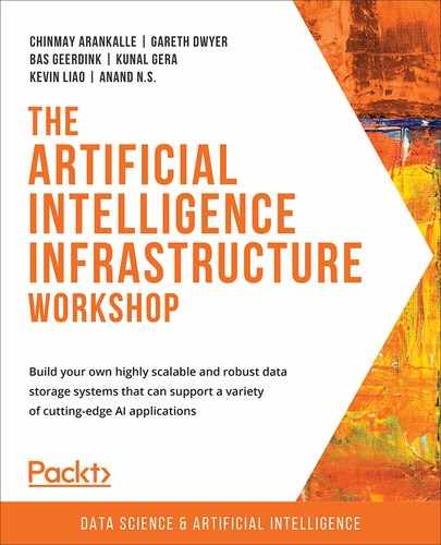
- Open your Terminal (macOS or Linux) or Command Prompt (Windows), navigate to the Chapter09 directory, and type jupyter notebook. The Jupyter Notebook should look as in the following screenshot:
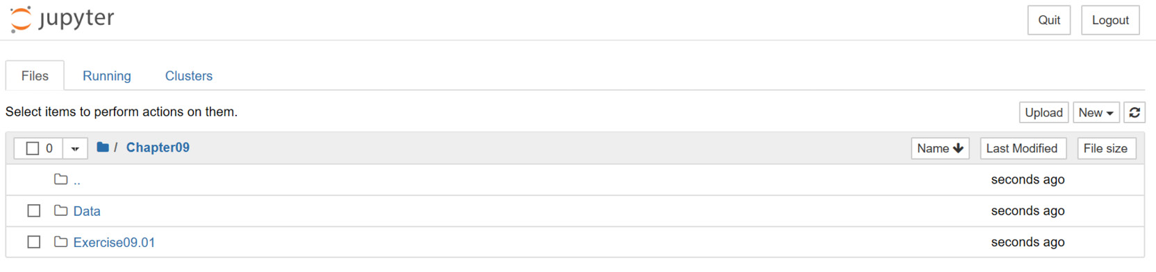
Figure 9.3: The Chapter09 directory in Jupyter Notebook
- Select the Exercise09.01 directory, then click New -> Python 3 to create a new Python 3 notebook, as shown in the following screenshot:

Figure 9.4: Create a new Python 3 Jupyter Notebook
- Import the pandas module and read the downloaded data using the read_csv method, as shown in the following snippet:
import pandas as pd
df = pd.read_csv('../Data/Usvideos.csv.zip' , compression='zip')
df.head()
You should get the following output:

Figure 9.5: A glimpse of US trending video data
- Filter the data for the date 17.14.11 by running the following command:
df.query('trending_date=="17.14.11" ')
You should get the following output:

Figure 9.6: US trending videos on the date 2017-11-14
- Create a get_trendy_vids.py Python script under the Exercise09.01 directory.
Note
Besides using Jupyter Notebook, we can also create a Python script in a Terminal with touch get_trendy_vids.py. Another recommended option is to use the Visual Studio Code as a text editor to write Python script.
- Write the following code inside the get_trendy_vids.py Python script:
from pathlib import Path
import pandas as pd
def get_topn_viewed(df, date, topn):
return df.query('trending_date==@date').sort_values('views', ascending=False).head(topn)
if __name__ == "__main__":
# config
PATH_FILE_IN = Path(__file__).parent.absolute()/'../Data/USvideos.csv.zip'
PATH_FILE_OUT = Path(__file__).parent.absolute()/'../Data/top_10_trendy_vids.c sv'
DATE = "17.14.11"
TOPN = 10
# read data
df_data = pd.read_csv(PATH_FILE_IN, compression='zip')
# get top n trendy
df_trendy = get_topn_viewed(df_data, DATE, TOPN)
# save results
df_trendy.to_csv(PATH_FILE_OUT, index=False)
The Python program sorts the views column in descending order. It then selects the top 10 trending videos for Nov 14, 2017 (17.14.11) and writes to a CSV file named top_10_trendy_vids.csv.
Note
We have separated the functions from the execution steps. The code under the if __name__ == "__main__": statement is executed in sequential order when you run this Python script. The functions defined in the previous step are registered as modules at the global level. This separation makes the code look cleaner and makes it easier for others to understand.
It's best to put all hardcoded variables at the beginning of the program so that they can be modified next time without having to go through all the code to change each value one by one.
- In your Terminal, navigate to the Exercise09.01 directory and run the following command to generate the top 10 trending videos:
python get_trendy_vids.py
The data for the top 10 trending videos are stored in a CSV file named top_10_trendy_vids.csv in the Data directory.
- Open the top_10_trendy_vids.csv file in Jupyter Notebook using the following command:
import pandas as pd
pd.read_csv('../Data/top_10_trendy_vids.csv')
You should get the following output:
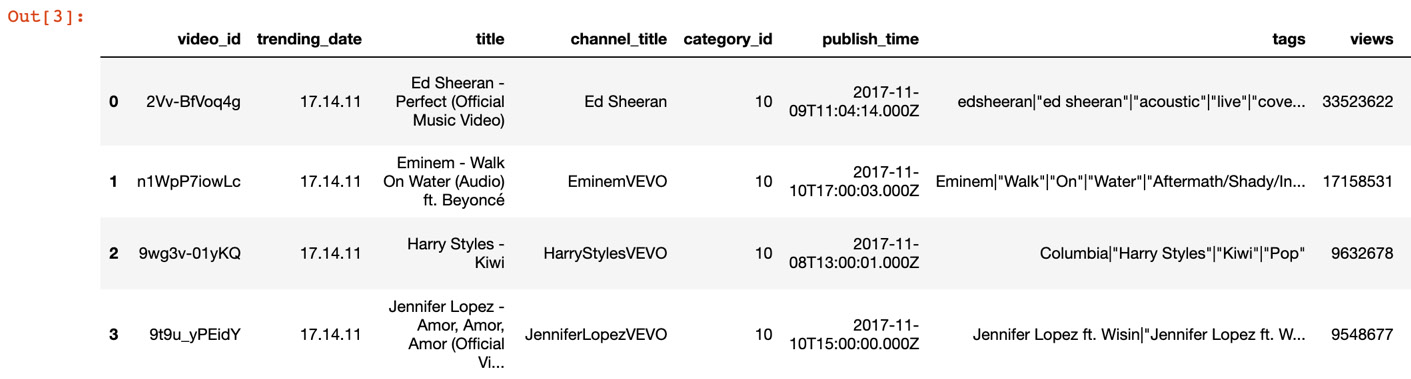
Figure 9.7: Top 10 trending US videos
We have successfully created a Python job to get the daily top 10 trending US videos.
Note
To access the source code for this specific section, please refer to https://packt.live/32eIzUm.
Note
We use Jupyter Notebook quite often during development. When we work with data, Jupyter Notebook is a great tool to understand and visualize underlying data and its structure. However, as great as Jupyter Notebook is as a development tool, it's best not to use it for production-level applications. It's preferred to use a Python script as the executable for a Python program.
Although the Python job we created in this exercise is very simple, we can still break it down into a multi-stage process. This is illustrated in the following figure:

Figure 9.8: A flow chart for fetching the top 10 trending videos
In our Python job, we first use pandas to read raw data, then we use the pandas DataFrame API to filter and sort data. Finally, we write the output data into a CSV file. These steps constitute a multi-stage process data pipeline.
By completing this exercise, you have successfully implemented your first data pipeline to generate the top 10 trendy US videos in Python using pandas. We implemented a three-step data pipeline in a single Python script. In the next exercise, we will expand our data pipeline and create a multi-stage pipeline with multiple Python scripts.
Exercise 9.02: Creating a Nonlinear Pipeline to Get the Daily Top 10 Trending Video Categories
In this exercise, we will increase the complexity of our data pipeline. We will build a pipeline that depends on two data sources: one is the same data from the previous exercise, while the other one is the video category data, which is stored in the US_category_id.json file. We will use both data sources to get information on the daily top 10 trending video categories.
During Exercise 9.01, Implementing a Linear Pipeline to Get the Top 10 Trending Videos, we found that there is a category_id column in the dataset, but it's an integer column. We want to find out the literal category for each YouTube video. This means we need to find out the mapping between the actual name of the category and the category ID. Now, your job is to create another Python program that generates the top 10 trending video categories.
Perform the following steps to complete the exercise:
- Create a new directory, Exercise09.02, in the Chapter09 directory to store the files for this exercise.
- Open your Terminal (macOS or Linux) or Command Prompt (Windows), navigate to the Chapter09 directory, and type jupyter notebook. The Jupyter Notebook should look as shown in the following screenshot:

Figure 9.9: The Chapter09 directory in Jupyter Notebook
- In the Jupyter Notebook, click the Exercise09.02 directory and create a new notebook file with the Python 3 kernel.
- We will use a built-in module, json, to load the JSON file as shown in the following code:
# read cat data
import json
cat = json.load(open('../Data/US_category_id.json', 'r'))
cat
You should get the following output:

Figure 9.10: YouTube video category data
The JSON file gets loaded into the Python environment as a dictionary object. We can see that there are three keys, ['kind', 'etag', 'items'], at the highest level. Within the items key, there is an array of sub-dictionaries. Within one of these sub-dictionaries, we can extract the title category from the snippet sub-key.
The category information is in the items key. The id key maps to category_id in the previous dataset, USvideos.csv.
- Create a pandas DataFrame out of the dictionary object (cat) using the following code:
import pandas as pd
df_cat = pd.DataFrame(cat)
df_cat
You should get the following output:

Figure 9.11: pandas DataFrame of YouTube video category data
- Now, extract title and id from the dictionary object and store them in the new category and id columns using the .apply function, as shown in the following code:
df_cat['category'] = df_cat['items'].apply(lambda x: x['snippet']['title'])
df_cat['id'] = df_cat['items'].apply(lambda x: int(x['id']))
df_cat
You should get the following output:

Figure 9.12: The new category and id columns
The category's title is stored under the snippet, which is stored under the item sub-dictionary as mentioned in Step 4. Similarly, the id category comes from the value of the id key. The pandas.apply function iterates rows along the item column and returns the value that we define in the lambda function.
- Drop the kind, etag, and items columns using the .drop function as shown in the following code:
df_cat_drop = df_cat.drop(columns=['kind', 'etag', 'items'])
df_cat_drop
You should get the following output:

Figure 9.13: Removed unnecessary columns
We have created a df_cat_drop mapping table from the JSON file successfully.
- Read the USvideos.csv.zip video data with pandas, then filter to trending_date=="17.14.11":
# read video data
df_vids = pd.read_csv("../Data/USvideos.csv.zip", compression='zip').query('trending_date=="17.14.11"')
We created a DataFrame called df_vids that contains information about each YouTube video and video category ID. We will join this DataFrame with df_cat_drop in the next step.
- Merge the df_cat_drop and df_vids DataFrames using the pandas.merge method, as shown in the following code:
# merge
df_join = df_vids.merge(df_cat_drop, left_on='category_id', right_on='id')[
['title', 'channel_title', 'category_id', 'category', 'views']]
df_join
You should get the following output:

Figure 9.14: The joined DataFrame from two datasets
By merging the two DataFrames, we now have category information for each YouTube video. The pandas .merge function merges two DataFrames when the category_id column from the left DataFrame, df_cat_drop, matches the value in the id column from the right DataFrame, df_vid.
We can use [["col_1", "col_2", …]] to select specific columns from the DataFrame. Here we selected the ['title', 'channel_title', 'category_id', 'category', 'views'] columns.
Now that we have a category for each YouTube video, we can group each category and sort them based on the total number of views for all of the videos.
- Group and sort the categories based on the total views using the .groupby function, as shown in the following code snippet:
df_join.groupby('category')[['views']].sum().sort_values('view s', ascending=False).head(10)
You should get the following output:

Figure 9.15: Top 10 most viewed YouTube video categories
In pandas, we can use pandas.groupby("column_1")[["column_2"]].sum() to calculate the sum of the values for each group. Furthermore, we can use pandas.sort_values("column", ascending=False) to re-rank the DataFrame.
The pandas.head(10) function will return the top 10 rows of the DataFrame.
- Now, create a get_trendy_cats.py Python script in the Exercise09.02 directory; we will combine all the preceding code snippets in it and save the file:
get_trendy_cats.py
1 import json
2 from pathlib import Path
3
4 import pandas as pd
5
6
7 def get_topn_categories(df, date, topn):
8 return df.query('trending_date==@date')
9 .groupby('category')[['views']].sum()
10 .sort_values('views', ascending=False).head(topn)
11
12
13 if __name__ == "__main__":
14 # config
15 PATH_FILE_VIDS = Path(__file__).parent.absolute()/'../Data/USvideos.csv.zip'
16 PATH_FILE_CAT = Path(__file__).parent.absolute()/'../Data/US_category_id.json'
17 PATH_FILE_OUT = Path(__file__).parent.absolute()/'../Data/top_10_trendy_cats.csv'
18 DATE = "17.14.11"
19 TOPN = 10
The full code is available at https://packt.live/2CpVXtL.
In the Python script, we first import libraries and define the get_topn_categories function to calculate the top (Most viewed) YouTube video categories. Under main, we use pandas to read the CSV file into a DataFrame. We also load the JSON file into a DataFrame and extract the category information. Then, we join them to get the joined DataFrame with category information. Finally, we calculate the top 10 most viewed YouTube video categories and save the file.
- Run the get_trendy_cats.py Python script as shown in the following code:
python get_trendy_cats.py
A new file, top_10_trendy_cats.csv, is created in the Data directory.
- Create a Python 3 Jupyter Notebook again and use the pandas.read_csv function to load the output for the top_10_trendy_cats.csv file, as shown in the following code:
# check data
pd.read_csv('../Data/top_10_trendy_cats.csv')
You should get the following output:
Figure 9.16: Top 10 YouTube video categories
Note
To access the source code for this specific section, please refer to https://packt.live/3fsb6t9.
We can represent the job in Exercise 9.02, Creating a Nonlinear Pipeline to Get the Daily Top 10 Trending Video Categories, as a multi-stage process. It looks like the following flow chart:
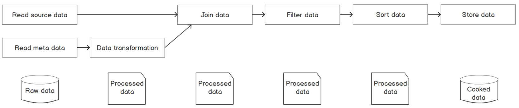
Figure 9.17: A flow chart for fetching the top 10 trending categories
We created a data pipeline that performs read, join, filter, sort, and store operations within a single Python script. Since all of the operations are in one single script, they are closely coupled together, which makes it less flexible and less reusable. In software engineering, a better practice is to write code in a more reusable and modular fashion so that it can be reused or recomposed to accomplish new tasks or larger tasks. In a later exercise, we will be creating a Python script for each operation.
Being able to break down a job into stages allows us to decouple different data operations. There are many benefits to decoupling data tasks. For example, it allows us to reduce code complexity for easier code maintenance. It also increases the overall robustness of the process. In Figure 9.3, let's imagine that the Filter data step fails. We would have to rerun the entire process from scratch. But if we decoupled each step and cached each step's output data, then we would just need to rerun the steps after the Join data step. Therefore, the system would be more manageable and more robust to failure events.
In the world of software engineering, the best practice for managing processes is to use a workflow application, commonly known as a workflow. A workflow is a software application that automates a process or processes to achieve a business-related objective. A process is usually composed of a series of steps to be automated. A workflow comes with many great features, such as automation, scheduling, failure handling, and the flexibility to allow users to introduce new components into an operation. You might wonder why we need a workflow and its awesome features to manage our processes. You will find out more about that in the next section.
Challenges in Managing Processes in the Real World
We have learned about how to create a task and break it into a multi-stage process. Knowing how to do these two things should be enough to create a functioning data pipeline. But when it comes to managing a data pipeline, there's another important thing to know about: job automation. Imagine that someone updated a source CSV file with the most recent data in the workflow illustrated in Figure 9.01. Someone would need to jump in to manually rerun the entire workflow and deploy a new version of the model.
Automation
To ease the burden of managing hundreds of workflows in a company, we want workflows to be fully automated without any extensive human interaction. If any change happens to one step, it should automatically trigger downstream steps to rerun with the new change. In addition to workflow automation, it'd be nice if we could version each run of the workflow so that we could perform retrospective analysis in the future:

Figure 9.18: A fully automated workflow
Failure Handling
Another consideration in managing workflows is failure handling. As great as a workflow is when fully automated, it can break. When one of the steps in a workflow breaks, it should not trigger downstream workflow steps. Otherwise, a defective model with potential bugs could be published to production, and we don't want that. For example, in Exercise 9.02, Creating a Nonlinear Pipeline to Get the Daily Top 10 Trending Video Categories, let's imagine the joining-data step fails and we end up re-ranking video categories based on the wrong values. In the end, we would publish an incorrect report to stakeholders. So, when we manage a workflow, we need to know the status of each step as well as each step's dependencies. A step gets triggered only if its upstream step's status is "successful run." On the other hand, when a step's status is "failure," its downstream step shouldn't run:

Figure 9.19: A workflow management system should have the notion of status
Retry Mechanism
Now, if a step's status is "failure," what should we do about it? A simple solution would be to have a re-try mechanism where the step will start running again after some pre-defined time window (for example, 60 seconds). When a pipeline is executing, it may encounter network issues that trigger pipeline failures. However, we don't want the pipeline to keep re-trying forever if there is a real issue that needs to be addressed; when we go to the ATM to withdraw cash, the card will be locked after three failed PIN attempts.
We can set it to re-try three times. If the step fails three times, then it will escalate to humans, which means we need the workflow management system to send out an email with reports to the engineers who own this workflow:
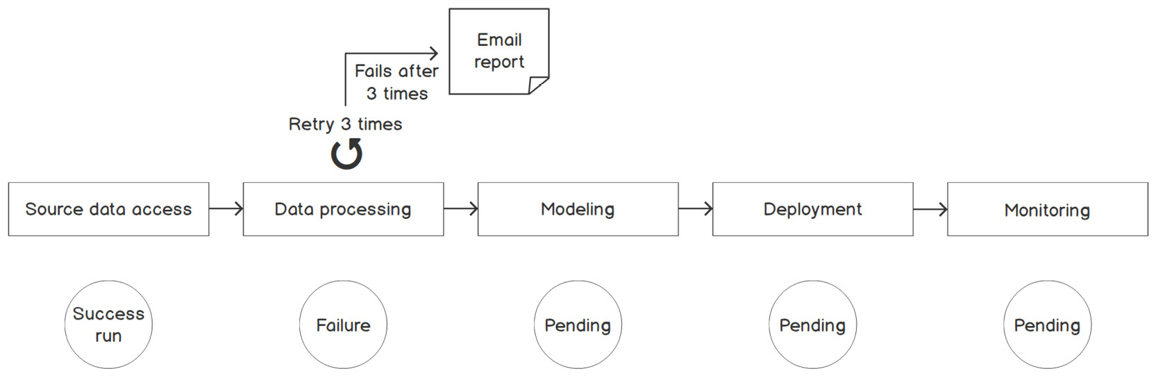
Figure 9.20: A workflow management system should have a re-try mechanism
In short, managing dependencies, scheduling the workflow, handling errors, versioning, and conducting retrospection are common challenges in the world of data science and AI. Many companies face the same pain points and have developed workflow management systems to tackle these problems. If you have experience in the realm of data engineering, these challenges may sound familiar to you. As soon as you start working with data, you will face these pain points and want to solve them.
To better understand why workflow management is needed in the real world, let's create a multi-stage data pipeline. A multi-stage data pipeline is composed of several individual tasks that have dependencies between them. The dependencies between tasks in a pipeline can be complicated and hard to manage. Meanwhile, it leads to an opportunity to optimize a poorly organized pipeline. In the next exercise, we will be building a multi-stage process based on the previous exercise.
Exercise 9.03: Creating a Multi-Stage Data Pipeline
Recall that in Exercise 9.02, Creating a Nonlinear Pipeline to Get the Daily Top 10 Trending Video Categories, we created a job that took two files as input and then output the top 10 daily trending video categories. The logic for the entire process sat inside a single Python script, which meant it was a single-step process. To increase the robustness and modularity of the process, we want to break it into multiple steps with files cached at different stages. Now your job is to write multiple Python scripts to represent different steps in the process and achieve the same objective of displaying the top 10 daily trending categories. The single-task process shown in Figure 9.14 will be converted to a multi-stage process composed of multiple Python scripts, as shown in the following figure:
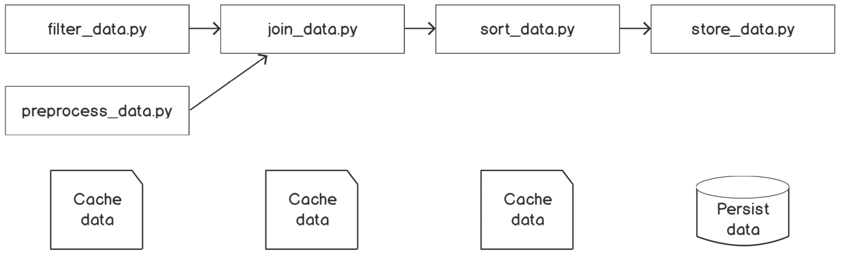
Figure 9.21: A multi-stage process composed of five different Python scripts
Perform the following steps to complete the exercise:
- Create an Exercise09.03 directory in the Chapter09 directory to store the files for this exercise.
- Open your Terminal (macOS or Linux) or Command Prompt (Windows), navigate to the Chapter09 directory, and type jupyter notebook.
- Create a filter_data.py Python script in the Exercise09.03 directory and add the following code:
filter_data.py
28 # filter
29 df_filtered = filter_by_date(df_data, date)
30 # cache
31 dir_cache = './tmp'
32 try:
33 df_filtered.to_csv(os.path.join(dir_cache, 'data_vids.csv'), index=False)
34 except FileNotFoundError:
35 os.mkdir(dir_cache)
36 df_filtered.to_csv(os.path.join(dir_cache, 'data_vids.csv'), index=False)
37 print('[ data pipeline ] finish filter data')
The complete code for this step is available at: https://packt.live/38U6v0c.
In filter_data.py, we write logic that reads source data from the file path where USvideos.csv.zip is located in your filesystem, then filters data to a specific date, such as 17.14.11. After the data is filtered, it should cache the temporary output file to a working space. In this case, our working space is a temporary directory named ./tmp/. The ./tmp/ directory will be our workspace for the rest of the data pipeline. Intermediate output files from other steps will be cached in this workspace as well. Other steps will use this workspace for read and write operations.
Note
We use the argparse module to create this program with a Command-Line Interface (CLI). A CLI enables users to run this program with various configurations without touching the code, which helps encapsulate the program.
- Create a preprocess_data.py Python script in the Exercise09.03 directory, and add the following code:
preprocess_data.py
19 # read data
20 data_cats = json.load(open(filepath, 'r'))
21 # convert json to dataframe
22 df_cat = pd.DataFrame(data_cats)
23 df_cat['category'] = df_cat['items'].apply(lambda x: x['snippet']['title'])
24 df_cat['id'] = df_cat['items'].apply(lambda x: int(x['id']))
25 df_cat_drop = df_cat.drop(columns=['kind', 'etag', 'items'])
26 # cache
27 dir_cache = './tmp'
28 try:
29 df_cat_drop.to_csv(os.path.join(dir_cache, 'data_cats.csv'), index=False)
30 except FileNotFoundError:
31 os.mkdir(dir_cache)
32 df_cat_drop.to_csv(os.path.join(dir_cache, 'data_cats.csv'), index=False)
33 print('[ data pipeline ] finish preprocess data')
The complete code for this step is available at: https://packt.live/306wPR2.
In preprocess_data.py, the program reads the video category data as a DataFrame from the file path where US_category_id.json is located. It then uses pandas.apply functions to extract the video category, title, and id from the item column. Finally, the program outputs the mapping table between the id and the title category to our workspace, ./tmp/.
- Create a join_data.py Python script in the Exercise09.03 directory, and add the following code:
import pandas as pd
def join_cats(df_vids, df_cats):
return df_vids.merge(df_cats, left_on='category_id', right_on='id')
if __name__ == "__main__":
import os
import sys
from os import path
# read data from cache
try:
df_vids = pd.read_csv('./tmp/data_vids.csv')
df_cats = pd.read_csv('./tmp/data_cats.csv')
except Exception as e:
print('>>>>>>>>>>>> Error: {}'.format(e))
sys.exit(1)
# join data
df_join = join_cats(df_vids, df_cats)
# cache joined data
df_join.to_csv('./tmp/data_joined.csv', index=False)
print('[ data pipeline ] finish join data')
In join_data.py, we map the id category from the YouTube video data to the title category from the data category. Notice that we did not use a CLI for this join step because this program depends on the completion of previous steps and assumes that input data has already been cached in the pipeline workspace, ./tmp/.
Note
The try … except block is recommended for use here because the program expects that data_vids.csv and data_cats.csv are available. When files are not available, which is not expected, we want this program to exit with status code 1 to tell the data pipeline to abort the operation as well as to print the error message.
- Create a sort_data.py Python script in the Exercise09.03 directory, and add the following code:
sort_data.py
1 import sys
2 import pandas as pd
3 import argparse
4
5 def get_topn_cats(df_join, topn):
6 return df_join.groupby('category')[['views']].sum()
7 .sort_values('views', ascending=False).head(topn)
8
9 def parse_args():
10 parser = argparse.ArgumentParser(
11 prog="exercise 3",
12 description="rank categories")
13 parser.add_argument('-n', '--num', type=int, default=10, help='how many?')
14 return parser.parse_args()
The complete code for this step is available at: https://packt.live/3iXdtq3.
In sort_data.py, the program reads the data_joined.csv file. Then, it sums up the video views for each category and ranks the categories in terms of total views in descending order to show the top 10 trending categories. We wrap the logic that performs the group-by sum operations in a function called get_top_cats. This will make the code more readable, reusable, and modular.
- Create a store_data.py Python script in the Exercise09.03 directory, and add the following code:
store_data.py
19 # read data from cache
20 try:
21 file_cached = './tmp/data_topn.csv'
22 df_join = pd.read_csv(file_cached)
23 except Exception as e:
24 print('>>>>>>>>>>>> Error: {}'.format(e))
25 sys.exit(1)
26
27 # cache joined data
28 df_join.to_csv(filepath, index=False)
29
30 # clean up tmp
31 shutil.rmtree('./tmp')
32
33 print('[ data pipeline ] finish storing data')
The complete code for this step is available at: https://packt.live/3frBJhP.
In store_data.py, the program will read the output file from the last step and write the file to a new location to persist the final output data from this pipeline. Since the final output data is persisted in a given location, the cached data that was created in the previous steps is no longer needed. At the end of the pipeline, we use the built-in shutil library to remove the ./tmp directory along with all the files inside it. This program's CLI requires an argument for the output file path in which users want to store the output data.
- Now, run the following commands in sequential order in your Terminal (assuming you are in the Exercise09.03 directory):
python filter_data.py --file ../Data/USvideos.csv.zip --date 17.14.11
You should get the following output:

Figure 9.22: Output of filter_data.py
python preprocess_data.py --file ../Data/US_category_id.json
You should get the following output:

Figure 9.23: Output of preprocess_data.py
python join_data.py
You should get the following output:

Figure 9.24: Output of join_data.py
python sort_data.py
You should get the following output:

Figure 9.25: Output of sort_data.py
python store_data.py --path ../Data/top_10_trendy_cats.csv
You should get the following output:

Figure 9.26: Output of store_data.py
A new top_10_trendy_cats.csv file is created in the Data directory.
- Open a new Python 3 Jupyter Notebook, import pandas, and use the read_csv function to read the top_10_trendy_cats.csv file, as shown in the following code:
import pandas as pd
pd.read_csv('../Data/top_10_trendy_cats.csv')
You should get the following output:
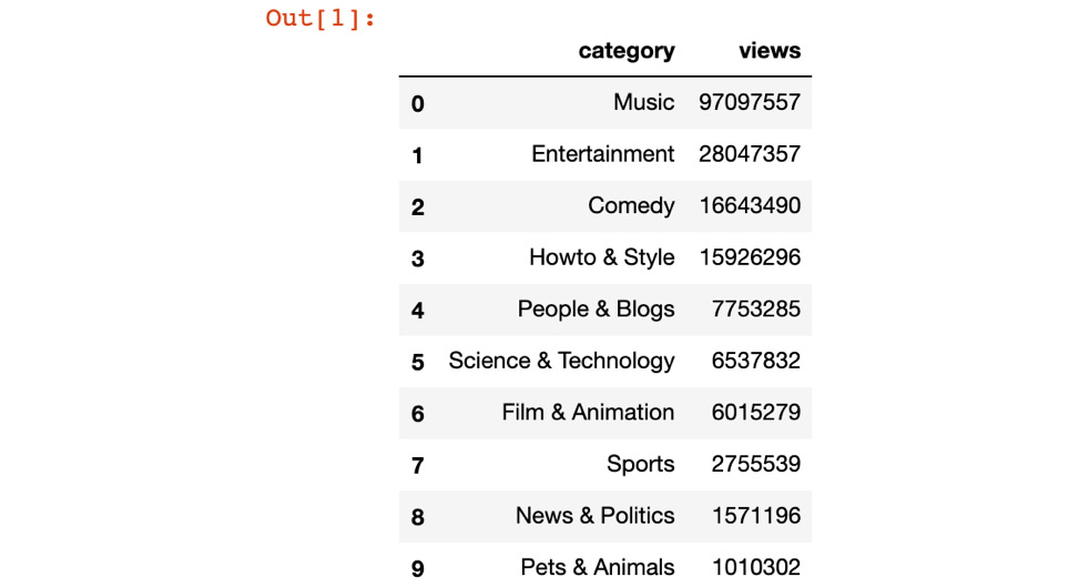
Figure 9.27: Top 10 most viewed video categories
Note
To access the source code for this specific section, please refer to https://packt.live/3emvKK0.
By completing the exercise, you have successfully implemented a multi-stage data pipeline that is composed of five Python scripts. Each Python script on its own is a modular and reusable operation. For example, the filter_data.py script implements the filter operation. Another script, preprocess_data.py, implements the preprocess operation. With more of these modular and reusable scripts for different types of data operations, we can pipe different operations together to compose any data pipeline we want.
Automating a Data Pipeline
You may think that multi-stage jobs are complicated. Users are required to run multiple commands in a specific sequence to complete tasks. One of the principles of workflow management is the minimization of human interaction. Human interaction is usually error-prone. If someone runs commands in the wrong order, there will be different results. We want to remove this manual process, which means we need to automate this job.
Bash is a Unix shell. It's a command language that can be used directly at the command line. Often, people use Bash as glue code to stitch different software systems or tools together, as well as using it for the automation of jobs.
In the next exercise, we will leverage Bash to automate the multi-stage data pipeline of Exercise 9.03, Creating a Multi-Stage Data Pipeline.
Exercise 9.04: Automating a Multi-Stage Data Pipeline Using a Bash Script
In the last exercise, we created four Python scripts, one for each stage of a multi-stage data pipeline. Furthermore, we ran each of them manually to store the data in a CSV file.
This exercise aims to automate the stages of the pipeline using a Bash script.
Perform the following steps to complete the exercise:
- Create a new Exercise09.04 directory in the Chapter09 directory to store the files for this exercise.
- Create a run_job.sh Bash script in the Exercise09.04 directory and add the following code:
run_job.sh
1 #!/bin/bash
2
3 set -e
4
5 # set config
6 DATE=17.14.11
7 SOURCE_FILE=../Data/USvideos.csv.zip
8 CAT_FILE=../Data/US_category_id.json
9 OUTPUT_FILE=../Data/top_10_trendy_cats.csv
10 SRC_DIR=../Exercise09.03
11
12 echo "[[ JOB ]] runs on date $DATE with file located in $SOURCE_FILE and metadata located in $CAT_FILE"
13 echo "[[ JOB ]] result data will be persisted in $OUTPUT_FILE"
The complete code for this step is available at: https://packt.live/32aF3Kw.
In the run_job.sh Bash script, the first line (as always) is #!/bin/bash to indicate that it's a Bash script. We use a Bash built-in command, set –e, to tell the Bash program to exit immediately if any command within the pipeline returns a non-zero status.
We also set a bunch of variables, DATE, SOURCE_FILE, CAT_FILE, OUTPUT_FILE, and SRC_DIR, at the top of the script.
The next lot of commands look similar to the commands used in Exercise 9.03, Creating a Multi-Stage Data Pipeline, for the sequential execution of our data pipeline. The only difference is the additional echo command, which writes messages to standard out. During the running of the Bash script, echo messages show us which step of the pipeline is currently running.
At the bottom of the script, the last six lines of code are making sure that the program exits with the appropriate status code. When the program exits with code 1, this means the program failed with an unexpected error. This increases the robustness of the system in terms of error-handling.
- Open your Terminal (macOS or Linux) or Command Prompt (Windows), navigate to the Chapter09/Exercise09.04 directory, and run the following command:
sh run_job.sh
You should get the following output:

Figure 9.28: A successful pipeline run in the Terminal via Bash
When we see the [[ JOB ]] END message, it means the Bash script ran until the end without returning a non-zero exit code. In other words, the pipeline is running successfully.
Now, we can check the output data that is saved in Chapter09/Data/top_10_trendy_cats.csv location.
- Open a new Python 3 Jupyter Notebook, import pandas, and use the read_csv function to read the top_10_trendy_cats.csv file, as shown in the following code:
import pandas as pd
pd.read_csv('../Data/top_10_trendy_cats.csv')
You should get the following output:
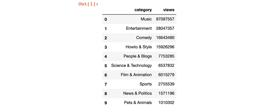
Figure 9.29: Top 10 most viewed video categories
By completing this exercise, we learned to use a Bash script to automate a multi-stage data pipeline. We used Bash script built-in commands and variables to store file path information and other parameters that are used in the pipeline. To log the status for each step in the pipeline, the echo command was used.
Bash is used as glue code to compose different operations together to control jobs, or in our case, to automate a job.
Note
To access the source code for this specific section, please refer to https://packt.live/3fqHpIO.
In Exercise 9.04, Automating a Multi-Stage Data Pipeline Using a Bash Script, when we ran the run_job.sh Bash script in Terminal, the program was executing each line in a sequence. The next line won't be executed until the current line is done. For example, the program won't run step 1.1 preprocess metadata until step 1 filter source data is finished. This is called synchronous execution. Because we ran this Bash script on our local machine with a single-thread process, by default it was a synchronous process. But step 1 and step 1.1 don't need to run in a specific sequence; they can run as parallel steps as well. The job will be more efficient if step 1 and step 1.1 can run at the same time, rather than running in sequence. This would make it asynchronous execution.
Most real-world applications are asynchronous processes, especially in the world of distributed computing. In a single cluster, many compute instances are executing different tasks at the same time to achieve efficient computing. But the next question for us is this: if a program is not executed in a synchronous manner, how can we automate this program? In the next section, we will discuss solutions for managing asynchronous data pipelines.
Automating Asynchronous Data Pipelines
A workflow management system should have the ability to automate asynchronous processes without any human interaction. Let's use the most common type of job in data engineering, the Extract, Transform, and Load (ETL) workflow, as an example to illustrate how it works and how to automate it:

Figure 9.30: A typical ETL workflow
The objective of an ETL pipeline is to output analytics reporting to inform business analysts what is trending right now based on clicks and impression data, which is very similar to the YouTube trending video data pipeline we created earlier. However, an ETL pipeline usually involves performing data operations such as extracting, transforming and loading data at scale.
Let's imagine that our source data, USvideos.csv.zip, is a 100+ terabytes dataset, which is very common in the era of big data. We won't be able to work with a flat CSV file anymore. Data of such size will be stored in specialized data systems such as the Hadoop Distributed File System (HDFS) and other cloud storage systems. The data won't be stored in a single file. It will be partitioned into many files so that the data is manageable as well as fault-tolerant. So, our data pipelines will have to read data from many sources simultaneously in the first step.
In the processing step of our data pipeline, pandas is no longer a viable option for processing data at such a scale. We will use a big data processing engine such as Spark, which is offered through Amazon Elastic MapReduce (EMR), to perform group, aggregation, and sort operations using the map-reduce paradigm.
At the end of the pipeline, the pipeline will persist the final output data to a location. In our example, the location is a cloud memory storage system, Amazon ElastiCache. It's a key-value store for fast access, and it will be talked about in more depth in the next chapter.
The process in Figure 9.21 is a typical ETL workflow, which usually involves extracting raw data from multiple data sources, transforming raw data into a digestible format, then loading the results into another data store.
Each step runs inside a compute instance. You can think of a compute instance as an independent self-contained environment with resources such as CPU and RAM that aren't shared with others. Notice that the first step in this ETL pipeline is very similar to that of the pipeline in Exercise 9.04, Automating a Multi-Stage Data Pipeline Using a Bash Script, where tasks in the first step didn't have dependencies with each other and were parallelized. Each task in the first step can be finished at a different time, but the second step won't be triggered until the last task in the first step is finished. So, this pipeline is an asynchronous process.
We need to introduce a new mechanism to understand the dependencies between tasks and be able to trigger the next task when its dependent tasks are completed.
There are multiple approaches to automating asynchronous processes. Let's look at one of them here:
- We need a mechanism that triggers downstream tasks in a workflow when a certain criterion is met. In this case, this mechanism checks for the user session data becoming available in AWS S3, then it will trigger the next task.
- We also need to make this mechanism understand the dependencies between tasks so that tasks get triggered in the intended sequence. Practitioners in the industry have figured out that the best way to define workflows with task dependencies is to use Directed Acyclic Graphs (DAGs). We will study DAGs later in this chapter.
Based on the two requirements, we need to add two more tasks to the workflow:

Figure 9.31: Adding two more tasks for workflow automation
Let's zoom in on the workflow again and take a look at the newly added tasks. We can see that the two new added tasks are different than the original tasks in nature. They act as a sensor and trigger as they sense whether a condition is met. While the first and fifth steps are simply moving data from one place to another, the third step is performing some actions on the data.
In workflow management, we use the term operator as a basic unit of abstraction to define tasks. A workflow is defined in a DAG and operators are nodes in the DAG that represent tasks. There are three types of operators: action, transfer, and sensor.
We can customize any workflow using these three operators. Most ETL workflows are constructed with these three operators. Here's a general illustration of how they function:

Figure 9.32: An ETL workflow using different types of operators
In the next exercise, we will further improve our data pipeline by introducing the use of asynchronous processes to speed up the runtime. With asynchronous processes, we also need to implement a sensor operation for triggering downstream operations in the pipeline.
Exercise 9.05: Automating an Asynchronous Data Pipeline
Let's try to implement the triggering (sensor operator) mechanism in the Bash script and automate the job in Exercise 9.04, Automating a Multi-Stage Data Pipeline Using a Bash Script.
Perform the following steps to complete the exercise:
- Create an Exercise09.05 directory in the Chapter09 directory to store the files for this exercise.
- Create a run_job.sh Bash script in the Exercise09.05 directory and add the following code:
#!/bin/bash
set -e
# set config
DATE=17.14.11
SOURCE_FILE=../Data/USvideos.csv.zip
CAT_FILE=../Data/US_category_id.json
OUTPUT_FILE=../Data/top_10_trendy_cats.csv
SRC_DIR=../Exercise09.03
echo "[[ JOB ]] runs on date $DATE with file located in $SOURCE_FILE and metadata located in $CAT_FILE"
echo "[[ JOB ]] result data will be persisted in $OUTPUT_FILE"
# run job
echo "[[ RUNNING JOB ]] step 1: filter source data"
python $SRC_DIR/filter_data.py --file $SOURCE_FILE --date $DATE &
echo "[[ RUNNING JOB ]] step 1.1: preprcess metadata"
python $SRC_DIR/preprocess_data.py --file $CAT_FILE &
echo "[[ RUNNING JOB ]] step 2: join data"
python $SRC_DIR/join_data.py
echo "[[ RUNNING JOB ]] step 3: rank categories"
python $SRC_DIR/sort_data.py
echo "[[ RUNNING JOB ]] step 4: persist result data"
python $SRC_DIR/store_data.py --path $OUTPUT_FILE
if [ "$?" = "0" ]; then
rm -rf ./tmp/
echo "[[ JOB ]] END"
else
rm -rf ./tmp/
echo "[[ JOB FAILS!! ]]" 1>&2
exit 1
fi
At first glance, run_job.sh looks the same as the script in Exercise 9.04, Automating a Multi-Stage Data Pipeline Using a Bash Script. But it's not the same – you'll notice the difference in the python $SRC_DIR/filter_data.py --file $SOURCE_FILE --date $DATE & and python $SRC_DIR/preprocess_data.py --file $CAT_FILE & commands. We added the & symbol at the end of the command line, which directs the shell to run the command in the background; that is, it runs in a separate sub-shell, as a job, asynchronously. When the first two commands in the pipeline are running in the background, Bash will immediately return the status code 0 for true. Once the status code 0 is returned, the next command starts to run. This means that the Bash script doesn't wait for the first two steps to finish but continues to execute the remaining commands in the script. You have probably noticed that this isn't a desirable behavior and will cause errors. We will find out its solution in the next step of the exercise.
- Open your Terminal (macOS or Linux) or Command Prompt (Windows), navigate to the Chapter09/Exercise09.05 directory, and run the following command:
sh run_job.sh
You should get the following output:
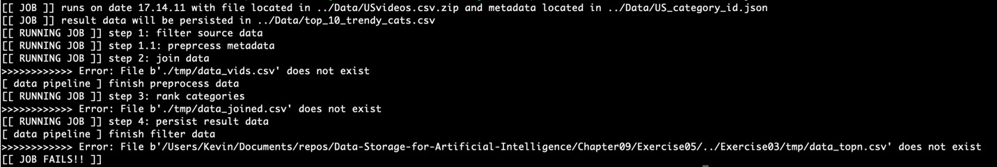
Figure 9.33: Pipeline error without a sensor operator
The error occurs in step 2 while running the join_data.py script. It's complaining about the data_vids.csv file not existing in the workspace. This is because step 1 filter_data.py hasn't finished executing and so the data_vids.csv file wasn't written to the ./tmp/ directory.
To solve this error, we need to implement a sensor operator. It will ensure that until the files are available, step 2 join_data.py is not triggered.
- In the run_job.sh Bash script, add the while construct (highlighted) before step 2 to implement the sensor operator as shown in the following code:
run_job.sh
22 echo "[[ BLOCKING JOB ]] additional step: check cached files and trigger next step"
23 while [ ! -f ./tmp/data_cats.csv ] || [ ! -f ./tmp/data_vids.csv ]
24 do
25 sleep 1
26 done
27
28 echo "[[ RUNNING JOB ]] step 2: join data"
29 python $SRC_DIR/join_data.py
30
31 echo "[[ RUNNING JOB ]] step 3: rank categories"
32 python $SRC_DIR/sort_data.py
33
34 echo "[[ RUNNING JOB ]] step 4: persist result data"
35 python $SRC_DIR/store_data.py --path $OUTPUT_FILE
The complete code for this step is available at: https://packt.live/32eKzfg.
The while loop code block acts as a sensor operator between steps 1 and 2. When the commands of step 1 are running in the background, it will check whether the data_cats.csv and data_vids.csv files are available in tmp/. If they're not found, it will sleep for 1 second and continue to check the while condition until the files are available. When the files are available, the Bash program will exit the while loop and execute the commands in step 2.
- Save the updated run_job.sh Bash script and run it again using the following command:
sh run_job.sh
You should get the following output:

Figure 9.34: A successful asynchronous pipeline run with a sensor operator
By completing the exercise, you have successfully implemented an asynchronous multi-stage data pipeline with a Bash script. We first learned how to use the & symbol in Bash to direct the shell to run a command in the background asynchronously. Then we implemented a while loop that acted as a sensor operator to block the step 2 commands until the step 1 commands had finished.
Note
To access the source code for this specific section, please refer to https://packt.live/3iXdYQX.
Now we can write a Bash program to automate not only synchronous jobs but asynchronous jobs as well. This is great if the job never fails. However, task jobs in real life can fail. Imagine that the tasks of step 1 kept failing; the program would be stuck at the [[ BLOCKING JOB ]] step and the rest of the steps would be blocked forever. We need more sophisticated mechanisms in a production-level workflow management system. A workflow management system should be able to monitor the life cycle and health of each task in each step as well as the overall status of the entire job.
It should be able to handle errors as well as re-try tasks. This is possible using Airflow, an open-source workflow management tool. In the next section, we will use the Airflow DAG API, to create a DAG for our data pipeline, and the Airflow Operator API, to implement different data operations for the tasks in our data pipeline. Also, using the Airflow scheduler, we will run our DAG and monitor our DAG's status using its UI.
Workflow Management with Airflow
So far, we have learned how to create data pipelines and different types of workflows, including linear and non-linear ones. We define and implement workflows in Python scripts and use Bash to automate workflows. However, that is not enough for us to be able to manage workflows on a large scale. We are going to take workflow management to the next level by solving the following problems:
- Can we find a standardized way to define workflow dependency instead of writing a customized Bash script?
- Can we define data operations with a consistent interface instead of writing a Python program with a customized CLI?
- Can we have a standardized way to log the pipeline's running status?
- Can we monitor a running workflow? Can we schedule workflows?
The answer to all of these problems is Airflow. Airflow is a horizontally scalable, distributed workflow management system that allows us to specify complex workflows using Python code. It is an open-source project developed at Airbnb and it has a growing open source community. It's very easy to use and it has great documentation, so it's a perfect tool for us to manage workflows at scale with.
When we use Airflow to manage jobs, we first need to describe the job with a DAG. A DAG is a collection of tasks organized in a specific order. A DAG describes how you want Airflow to run your workflow. For example, you may want your workflow to run every day until the year 2021, or you may want Airflow to send you an email if the workflow fails, and so on. The DAG is there to make sure your workflow runs at the right time and in the right order, and that it handles errors whenever needed.
Let's consider the following workflows:

Figure 9.35: DAG and non-DAG workflows
Which workflow is described with a DAG? Only workflow (c) is using a DAG. Workflow (a) and (b) are cyclic workflows. It's very challenging to automate cyclic workflows because circular dependency causes infinite execution loops.
In the preceding charts, the DAG doesn't describe what A, B, C, D, E, and F are or what they are doing. A DAG doesn't concern itself with what the workflow is doing. It doesn't concern itself with each step or task. When we define a workflow, we also need to describe what the job should be doing with operators. An operator describes a single task in a workflow. It's usually atomic and can stand on its own. Airflow provides operators for most common tasks, such as BashOperator, PythonOperator, Sensor, and others.
In the next exercise, we will get our hands dirty with Airflow and create a DAG as well as operators for our data pipeline.
Exercise 9.06: Creating a DAG for Our Data Pipeline Using Airflow
Now that we have learned about Airflow, a powerful piece of open-source software for managing our workflow, let's start to write a DAG Python file for the workflow we created in previous exercises to generate daily top 10 trending video categories.
Before proceeding to the exercise, we need to set up Airflow in the local-dev environment. Please follow the instructions in the Preface to install it.
Perform the following steps to complete the exercise:
- Create an Exercise09.06 directory in the Chapter09 directory to store the files for this exercise.
- Open your Terminal (macOS or Linux) or Command Prompt (Windows), navigate to the Chapter09 directory, and type jupyter notebook.
- Create a top_cat_dag.py DAG Python script in the Exercise09.06 directory and add the following code:
Note
A DAG Python script should be named with _dag as a suffix; it's a convention in Airflow. This will help Airflow recognize it as a DAG file and register it in its metadata store.
import json
import os
import shutil
import sys
from datetime import datetime
import pandas as pd
from airflow import DAG
from airflow.operators.python_operator import PythonOperator
def filter_data(**kwargs):
# read data
path_vids = kwargs['dag_run'].conf['path_vids']
date = str(kwargs['dag_run'].conf['date'])
print(os.getcwd())
print(path_vids)
df_vids = pd.read_csv(path_vids, compression='zip')
.query('trending_date==@date')
# cache
try:
df_vids.to_csv('./tmp/data_vids.csv', index=False)
except FileNotFoundError:
os.mkdir('./tmp')
df_vids.to_csv('./tmp/data_vids.csv', index=False)
def preprocess_data(**kwargs):
# read data
path_cats = kwargs['dag_run'].conf['path_cats']
data_cats = json.load(open(path_cats, 'r'))
# convert json to dataframe
df_cat = pd.DataFrame(data_cats)
df_cat['category'] = df_cat['items'].apply(lambda x: x['snippet']['title'])
df_cat['id'] = df_cat['items'].apply(lambda x: int(x['id']))
df_cat_drop = df_cat.drop(columns=['kind', 'etag', 'items'])
# cache
try:
df_cat_drop.to_csv('./tmp/data_cats.csv')
except FileNotFoundError:
os.mkdir('./tmp')
df_cat_drop.to_csv('./tmp/data_cats.csv')
def join_data(**kwargs):
try:
df_vids = pd.read_csv('./tmp/data_vids.csv')
df_cats = pd.read_csv('./tmp/data_cats.csv')
except Exception as e:
print('>>>>>>>>>>>> Error: {}'.format(e))
sys.exit(1)
# join data
df_join = df_vids.merge(df_cats, left_on='category_id', right_on='id')
# cache joined data
df_join.to_csv('./tmp/data_joined.csv')
def sort_data(**kwargs):
topn = kwargs['dag_run'].conf.get('topn', 10)
try:
df_join = pd.read_csv('./tmp/data_joined.csv')
except Exception as e:
print('>>>>>>>>>>>> Error: {}'.format(e))
sys.exit(1)
# sort data
df_topn = df_join.groupby('category')[['views']].sum()
.sort_values('views', ascending=False).head(topn)
# cache joined data
df_topn.to_csv('./tmp/data_topn.csv')
def store_data(**kwargs):
# read data from cache
path_output = kwargs['dag_run'].conf['path_output']
try:
df_join = pd.read_csv('./tmp/data_topn.csv')
except Exception as e:
print('>>>>>>>>>>>> Error: {}'.format(e))
sys.exit(1)
# cache joined data
df_join.to_csv(path_output)
# clean up tmr
shutil.rmtree('./tmp')
Remember that a DAG is composed of data operators. In our case, we have data operations such as filter data, preprocess data, join data, sort data, and store data. In Airflow, we pass data operations to the DAG using Airflow's PythonOperator. When we define PythonOperator, we need to pass it a Python callable object, which is simply a Python function. So, the functions in the code will be used to create PythonOperator in later steps.
- Add the following code to the top_cat_dag.py script to create DAG:
# create DAG
args = {
'owner': 'Airflow',
'description': 'Get topn daily categories',
'start_date': datetime(2017, 11, 14),
'catchup': False,
'provide_context': True
}
dag = DAG(
dag_id='top_cat_dag',
default_args=args,
schedule_interval=None,
)
When we instantiate a DAG object, it requires dag_id, schedule_interval, and args. We create an args dictionary object first, then we create the DAG using args.
- Add the following code to the top_cat_dag.py script to create the PythonOperator instance to compose a real workflow:
op1 = PythonOperator(
task_id='filter_data',
python_callable=filter_data,
dag=dag)
op2 = PythonOperator(
task_id='preprocess_data',
python_callable=preprocess_data,
dag=dag)
op3 = PythonOperator(
task_id='join_data',
python_callable=join_data,
dag=dag)
op4 = PythonOperator(
task_id='sort_data',
python_callable=sort_data,
dag=dag)
op5 = PythonOperator(
task_id='store_data',
python_callable=store_data,
dag=dag)
When we instantiate a PythonOperator object, we need to give it a task_id argument, a unique namespace that distinguishes it from other operations. It also requires a python_callable argument, a Python function that defines the data operation. We also need to provide the DAG object to attach this PythonOperator to the DAG.
- Add the following code to the top_cat_dag.py script to add dependency information for the DAG:
[op1, op2] >> op3 >> op4 >> op5
We use Python bit shift operators to define a dependency between operators. You can tell that the bit shift operator points to downstream tasks. Operators being in brackets, [], means that they are parallel and not dependent on each other. In our case, operators 1 and 2 can be run in parallel first. When operators 1 and 2 are finished, operator 3 is allowed to run. When operator 3 is finished, then it will run operator 4. The same goes for operator 5.
- After completing the steps, the top_cat_dag.py DAG script should have the following code:
top_cat_dag.py
87 # create DAG
88 args = {
89 'owner': 'Airflow',
90 'description': 'Get topn daily categories',
91 'start_date': datetime(2017, 11, 14),
92 'catchup': False,
93 'provide_context': True
94 }
95
96 dag = DAG(
97 dag_id='top_cat_dag',
98 default_args=args,
99 schedule_interval=None,
100 )
101
102 op1 = PythonOperator(
103 task_id='filter_data',
104 python_callable=filter_data,
105 dag=dag)
The complete code for this step is available at https://packt.live/38Ypua7.
We first import several Python built-in functions and Airflow functions. In the DAG script, after the module import section, we define data operations for the data pipeline. In the second section of the DAG script, we define the DAG and its PythonOperators as well as the operator dependency.
Note
In the DAG script, we set 'provide_context': True in the args argument to instantiate the DAG. This will allow us to pass parameters to the DAG's operators when we trigger the DAG to run. You will notice this in the following steps.
- Run the following commands line by line in your Terminal:
# airflow needs a home, ~/airflow is the default,
# but you can lay foundation somewhere else if you prefer
# (optional)
export AIRFLOW_HOME=~/airflow
# install from pypi using pip
pip install apache-airflow
# initialize the database
airflow initdb
# start the webserver, the default port is 8080
airflow webserver -p 8080
# start the scheduler
airflow scheduler
# visit localhost:8080 in the browser and enable the example dag in the home page
If you have already installed Airflow, then you can skip the first two commands, $ export AIRFLOW_HOME=~/airflow and $ pip install apache-airflow. If this is the first time that you are using Airflow, you should run the $ airflow initdb command to initialize the Airflow database. It only needs to be run the first time. The $ airflow webserver -p 8080 command is used to launch the Airflow UI, which provides users with a graphical interface to interact with Airflow systems. The $ airflow scheduler command is used to launch the scheduler, which is responsible for getting your pipelines running on your local dev machine. The scheduler is required if you want to trigger DAGs to run.
Note
Please continue to stay in the same working directory, Exercise09.06, while you are launching Airflow because Airflow will treat your current working directory as its working directory. Later, our file path locations are based on this working directory. If you are using another working directory, you may get a file not found error.
When you launch an Airflow scheduler and it throws an attempt to write a readonly database error, it means the user who launched the Airflow scheduler does not have write permission to the Airflow SQLite database file, airflow.db. One way to resolve the permission issue is to issue the sudo chmod 644 ~/airflow/airflow.db command in your terminal and restart the Airflow scheduler. Run the following command to copy your DAG script to the Airflow home directory:
cp . /top_cat_dag.py ~/airflow/dags/
For Airflow to register the DAG in its system, we need to put the top_cat_dag.py DAG file in the Airflow home directory, ~/airflow/dags.
Note
The Airflow webserver and scheduler should be stopped when you copy a DAG script to ~/airflow. We can stop them by using Ctrl + C in the Command Prompt for Windows/Linux or Cmd + C for macOS. After the DAG script has been moved to the Airflow home directory, ~/airflow, we can launch the Airflow scheduler and webserver again. When the Airflow scheduler is launched again, it will register new DAGs from the DAG scripts in its home directory, ~/airflow. So, when we issue the airflow list_dags command, we can see the new DAGs that were added.
- Run the following command to list all the DAGs:
airflow list_dags
You should get the following output:

Figure 9.36: List of DAGs that are registered in your Airflow system
Airflow also supports the use of the CLI. Its CLI syntax is as follows: airflow action [options]. The list_dags action lists all of the available DAGs that are registered in the system. Notice that our DAG, top_cat_dag, is second from the bottom.
- Run the following command in the Terminal to trigger our DAG:
airflow trigger_dag -c '{"path_vids": "../Data/USvideos.csv.zip", "path_cats": "../Data/US_category_id.json", "date": "17.14.11", "path_output": "../Data/top_10_trendy_cats.csv"}' 'top_cat_dag'
The trigger_dag action will trigger the DAG to run immediately. The CLI requires the DAG ID, top_cat_dag. However, there is also a -c positional argument, which is for passing parameters into each operator in our DAG.
- To check the status of your DAG, you need to open your browser and go to http://localhost:8080/ to open the UI of the Airflow system. Look for the top_cat_dag DAG and click the Graph View icon, as shown in the following figure:

Figure 9.37: Our DAG information is shown in the Airflow UI
- Now, view the log of any task by clicking on the task and clicking the View Log button as shown in the following figure:

Figure 9.38: Monitoring the DAG's status
By completing this exercise, you have successfully implemented a DAG in Airflow as well as having completed the successful running of a workflow. A DAG is essentially a standardized interface for expressing a multi-stage data pipeline. We first created the DAG object. Then, we implemented our data operations with Airflow using PythonOperator. We also learned how to use Python bit shift operators to define dependencies in a workflow. After the DAG script was finished, we launched the Airflow UI and scheduler and got our DAG registered with Airflow. Lastly, we successfully triggered our DAG to run and finish.
Now we can launch Airflow as a workflow management system to automate our workflows as well as to use for monitoring purposes. But we have just started to scratch the surface of what Airflow can do. There are more features that we can explore in Airflow.
Note
To access the source code for this specific section, please refer to https://packt.live/2On0D6t.
In the next activity, we will be synthesizing everything we have learned in this chapter and composing a new workflow using Airflow.
Activity 9.01: Creating a DAG in Airflow to Calculate the Ratio of Likes-Dislikes for Each Category
Imagine that you are making a YouTube video and you want to optimize the number of likes you receive. You'd like to find out which YouTube video category tends to have more "likes" than "dislikes" So, you decide to find the likes-dislikes ratio based on various categories, such as sports, music, comedy, and so on. Depending on the findings, you will create your video.
In the YouTube video dataset, USVideos.csv.zip, there is a likes column and a dislikes column for each YouTube video. The table is shown here:

Figure 9.39: The likes and dislikes columns from the YouTube video data
This activity aims to find out the average ratio of likes to dislikes for each video category. You will need to first sum up likes and dislikes for each category. Then, you will calculate the likes-dislikes ratio for each category. Finally, you will write the result to a CSV file.
Note
The code and the resulting output for this activity can be found in a Jupyter Notebook here: https://packt.live/32puIdZ.
Perform the following steps to complete the activity:
- Read the USvideos.csv and US_category_id.json files using the pd.read_csv and json.load functions respectively.
- Extract the required columns using a DataFrame and a dictionary object.
- Join the DataFrames using the merge function and display the file using the head function:

Figure 9.40: YouTube video data with category information
- Calculate the total likes and dislikes grouped by category using the groupby function.
- Create a new ratio_likes_dislikes column and calculate the ratio by dividing the likes by the dislikes.
- Create a ratio_dag.py DAG script and add the required code in it.
- Register the DAG by copying the file into the Airflow Home directory and verify it using the list_dags command.
- Launch Airflow and trigger the DAG file using the trigger_dag command.
- Launch the Airflow UI using the Airflow webserver command.
- In the browser, check the status of the ratio_dag file using the Graph View icon.
- List the files in the ../Data/ directory and run the Ratio_Likes_Dislikes.csv file to get the following output:

Figure 9.41: Ratio of likes to dislikes for each category
Note
The solution to this activity can be found on page 634.
Summary
This chapter covered many concepts of workflow management and job control. We started by creating a simple data workflow with a single Python script. We then added more steps into the workflow and broke the workflow down into a multi-stage workflow. Next, we used Bash to compose as well as automate workflows. Lastly, we studied DAGs and implemented them using the open-source tool Airflow.
With the concepts and techniques that you have learned in this chapter, you will be able to tackle more sophisticated problems in the areas of AI and data science. Moreover, you will continue to learn and build experience on top of what you have gained from this chapter.
In the next chapter, you will learn about data solutions from public cloud providers such as Amazon Web Services. The concepts of implementing data operations and creating a data pipeline will be our building blocks for the next chapter. We will continue to build more sophisticated data storage solutions for use in AI and data science.