
In this chapter, you will learn about how ethics relate to Artificial Intelligence (AI) by looking at some of the largest industry scandals where AI ran up against morality. We will dive deep into several case studies, examining everything from AI being used to manipulate elections to AI displaying racial and sexist prejudices. We'll implement a simple sentiment classifier to differentiate between positive and negative words and sentences. We'll observe how this works in many cases and display the problematic biases and human stereotypes in the classifier. We'll gain hands-on experience with word embeddings and see how word embeddings can be used to represent how certain words relate to each other.
By the end of this chapter, you'll have learned how to evaluate the ethical aspects of the AI systems you build. You will know how to examine the potential consequences of using AI-based systems, and you'll know where to dive deeper to look for potential ethical problems. You'll be able to identify appropriate problems where word embeddings might be useful, and you'll be able to use Python's spaCy library for some common natural language processing (NLP) tasks.
Introduction
In the previous chapter, you learned how to prepare data using extract, transform, and load (ETL) pipelines to feed it efficiently into an AI system. In contrast, in this chapter, we'll take a break from looking at how things could be done, and we'll start asking whether they should be done. As with many new fields, AI has run up against ethical considerations. Ethics itself is always a topic that sparks controversy but combine that with a field that people often still associate with killer robots, and you're bound to find some very difficult and hotly debated topics.
Even outside of AI, robots can get into ethical trouble. For example, in 2014, the artistic group "!Mediengruppe Bitnik" created an automated trading bot that could buy random items from the so-called "dark web." The dark web is like the world wide web that most of us use every day, but you will not find its pages indexed on search engines such as Google. Instead, pages on the dark web hide behind specialized software, making sure that only specific people who are in the know can access them.
This dark web is often associated with illegal marketplaces, and people infamously trade illegal substances and weapons and run even darker marketplaces. The most widely publicized of these was known as "Silk Road," and it was shut down several times by authorities between 2013 and 2014.
!Mediengruppe Bitnik's bot was given a daily budget of $100, which was used to purchase random items and ship them to be exhibited as part of an art display. Of course, the bot's random purchases soon included an unsavory assortment of things, including illegal ecstasy tablets. In a highly publicized case, the world had to decide whether the bot itself had done something illegal or the creators of the bot had done something illegal.
After some legal debate, the police concluded that the purchases were in the name of "art" and were therefore not illegal, mainly because the artists never intended to sell or consume the illegal substance. The robot (the hardware running the AI) and its purchases were temporarily seized by the police but eventually returned. An exception was the MDMA tablets the robot had bought, which were destroyed. Overall, it was decided that it is acceptable to push boundaries in the name of art.
But what about the hundreds of companies using AI in similarly controversial ways for non-artistic purposes? There have been several high-profile cases over the past several years, and in this chapter, we will go through several case studies, examining some of the highest-profile cases where ethics and AI became a talking point.
Specifically, we will look at the following:
- The Cambridge Analytica scandal: This was where a private company helped a range of clients, from businesses to politicians, achieve their goals through AI and gained access to a vast trove of highly personal data via Facebook. It is widely believed that this was used to influence democratic elections, potentially bringing into question the validity of global democratic processes.
- Amazon's AI recruiting tool: This was where Amazon experimented with using AI to help it decide who to hire. It turned out that the algorithm displayed strong biases, specifically preferring male candidates over female ones. Amazon claims that it never used this tool for hiring purposes, but the fact that such a tool can exist makes us question whether other companies might have blindly depended on similar automated decisions without noticing built-in biases.
- COMPAS software and racist AI: This was the case of an algorithm that was used by US courts to predict whether prisoners are likely to commit further crimes being found to be biased against black people. A report in 2016 by ProPublica found that the algorithm made mistakes regarding black people twice as often as for whites, often incorrectly assessing black people as having a high "risk of re-offending."
The overall themes of these case studies are causing political harm at a country or global level via privacy invasion, causing social and financial harm through gender biases, and causing direct harm to individuals through the miscarriage of justice due to racial biases:
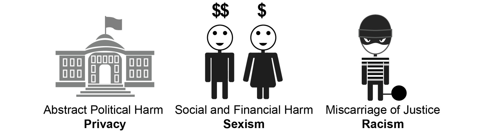
Figure 4.1: AI can display political, sexist, and racist biases
Let's get started by looking at a large, recent scandal: Cambridge Analytica.
Case Study 1: Cambridge Analytica
Cambridge Analytica Ltd (CA) was in the headlines of all major news publications for months after it became apparent that they, as a company, had used personal data to drive mass targeted campaigns, aiming to influence political elections. But how exactly did they use data? How did they use AI? And how does this relate to ethics?
Let's take a look at how Cambridge Analytica broke trust, and probably the law, through the following actions:
- Mass storage of personal data
- Invading people's privacy through mass collection and aggregation of data that would have been harmless in isolation
- Using AI to categorize the resulting mass of personal data and to identify specific groups of people who could be influenced in specific ways
- Using AI further to target specific advertisements at these groups to influence the way that they voted in elections
There is still much controversy, debate, and investigation concerning exactly what Cambridge Analytica did, how much they did it, and how effective it was. Some people claim that the story was overblown and that targeted advertising does not work that well in any case.
However, it certainly seems probable that there was a large and concerted effort to use data and AI for what many people would regard as "evil"—subverting political systems for financial gain.
Let's take a look at exactly how this might have worked.
With over 2.5 billion monthly active users, Facebook is perhaps the largest centralized store of personal data ever collected. A lot of this data is innocuous enough: someone's gender, their date of birth, where they live, and what they are interested in. More interestingly, Facebook also stores who everyone is friends with, how often they interact with each other, what brands and organizations they "like," what events they go to, and much more besides.
Many third-party companies gain access to subsections of this data via Facebook games, quizzes, and applications. These are small pieces of software that interact with your Facebook account in some way and require some of the personal data to work. Due to Facebook's popularity, these pieces of software have sometimes been political, with quizzes titled "Which political party are you most aligned with?" and similar, and this has often been useful for statistical and scientific research.
The value of this data also presents a business opportunity, though. Politicians need votes, and they spend large amounts of time and money trying to convince people to vote for them. Any politician or political party can broadly divide a population up into three groups:
- Strong supporters who will almost definitely vote for them, no matter what
- Strong opposers, who will almost definitely not vote for them, no matter what
- Moderates, who will follow events and opinions closely in the months and weeks leading up to an election and choose whether or not to vote for them based on these factors:

Figure 4.2: Strong supporters, strong opposers, and moderates
It is the last group, the moderates, who are the most interesting for politicians to spend time and effort trying to persuade. And one way to do this is through targeted digital advertising. Unlike advertising via traditional media, in which a politician pays to show the same advert to all readers, digital advertising allows for targeted advertising. This means that politicians can, in theory, show adverts only to the moderates, or people who might vote either way.
Additionally, they can further subdivide the moderates' group into different categories and show them each advert that would be more meaningful to their own beliefs. For example, young women with an interest in feminism might be a subgroup that can be influenced by hearing more about the politicians' plans to close the gender wage gap. Older males who have previously served in the army might be influenced by hearing more about politicians' plans to alleviate the financial hardship that many veterans face. Instead of creating a single campaign to try to find common interests in all groups, politicians can easily put on a "different face" when targeting each group.
It is not proven, but many now accept that voters can be manipulated by being shown targeted adverts relating to topics about which they are specifically sensitive. If this is true, the consequences are worrying. Do we want to live within a political system where the politicians with a digital marketing team and the best access to personal data are those who are voted into power?
Cambridge Analytica, by most accounts, created their innocuous-looking political quiz. To take the quiz, Facebook users had to allow the quiz software access to their private information. On top of this, Cambridge Analytica used a specific weakness in Facebook's Graph API to retrieve not only more personal information than might be expected from people who took the quiz, but also the same information from friends of people who took the quiz.
Using this treasure trove of personal data, Cambridge Analytica was able to use AI to not only categorize people into specific political affiliation groups and personality subtypes but also to effectively predict what kind of advertisement would sway these people to vote for their clients.
Knowing someone's birthday would not have been helpful for this kind of influence, and people know that their birthdays are not really private information and willingly give them out.
Knowing someone's location would similarly not have been helpful, and again, people are not guarded about sharing where they live.
The same goes for other individual bits of information, such as political leanings, favorite brands, events, and acquaintances. Bits of data on their own are not that interesting, but with enough data, and enough understanding of how the bits of data are connected, we start to derive information:

Figure 4.3: Data is only valuable when it is connected to other data in a meaningful way
But gathering all of this information about one person starts to paint a very specific picture. Imagine we know the following facts about an anonymous person:
- He is a 30-year-old male Facebook user.
- He has been to a Trump rally and a lecture by Bernie Sanders.
- He lives in the US in a state known to be a "battleground" or "swing" state.
- He has a large network of friends, many of whom match a similar profile.
- He often posts statuses that seem to be persuasive or argumentative in nature.
- His posts get an above-average number of likes and comments.
This person might be a prime candidate for targeted advertising. He is probably politically undecided, looking at arguments from both sides; in a position to influence many other people to match his views; and is located in a state that has better than average chances of being influential in the final election outcome.
Knowing a lot of basic information about some people or knowing some information about a lot of people wouldn't help Cambridge Analytica or their political clients. But knowing a lot of basic information about a lot of people is powerful. By looking at these facts and how they connect, it is possible to build a huge "knowledge graph" of information. Such a graph links people to facts, beliefs, and each other, and it can be used to manipulate them and therefore exert control over the world. We can use this information in combination with AI systems to help target specific messages at specific people:
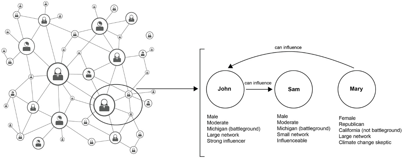
Figure 4.4: A knowledge graph – a huge collection of facts and connections can be used to train AI
How much data did Cambridge Analytica collect? While exact figures are hard to prove, the CEO claimed in 2016 that they had "four or five thousand" data points on every adult in the United States. Related specifically to the Facebook scandal, Cambridge Analytica claimed that they collected data from only 30 million Facebook profiles, but it was later confirmed that this number was closer to 87 million, with a large majority of these being from the USA.
Facebook lost a collective $100 billion due to a drop in share price after the scandal emerged in 2018, and further received a $5 billion fine from the Federal Trade Commission.
These numbers are scary. Data privacy laws are still catching up with what is possible to do through global aggregation and analysis of this type of data, so where laws fall short, we have to look to ethics to keep people and corporations in check.
One major ethical problem with this kind of use of personal data is that it relies on ignorance. Many people who use Facebook and the third-party software add-ons, such as the Cambridge Analytica quiz, do not realize that this kind of use of their data is possible. Therefore, while they may have agreed to let the quiz app access their data, this is not an informed choice. Imagine the following scenario based on the preceding knowledge graph:
- John is an active user of Facebook. He does not care about privacy and does not understand why his data might need to be kept private. He installs many apps and quizzes on Facebook (including the Cambridge Analytica one) and clicks "agree" on the notifications about the terms and conditions and privacy policy without reading them.
- John is Facebook friends with Mary. Mary is very privacy-aware. All of the personal information associated with her Facebook profile is set so that only her friends can see it. She understands the implications of making personal data public, and she never installs any apps or quizzes on Facebook.
- Because John installed the Cambridge Analytica quiz, it can use his account on behalf of him and can see everything he can see. Therefore, Cambridge Analytica can now see all of Mary's data too, even though she took measures to prevent this. While in this case, Cambridge Analytica might have obtained legal consent (via John), many people would argue that this is an ethical privacy violation from Mary's point of view.
Perhaps a more serious ethical problem is that this kind of use of data has the potential to undermine (or, depending on who you talk to, has already undermined) our entire global political system. Most countries today rely on some form of democracy—a form of government that strongly depends on all citizens having unbiased access to accurate information. If the political side with the larger checkbook and the better marketing team can influence specific groups of people by overloading them with evocative one-sided information, democracy as a system ceases to work as it is intended to work.
Summary and Takeaways
In this case study, we saw how Cambridge Analytica built a system that used mass data storage and AI to collect personal information from a lot of people without their informed consent. It further allegedly used this information to present potential voters with biased information, specifically targeting certain groups and individuals with adverts that were more likely to influence them.
This has large implications not only for our right to personal privacy but also for our political systems, which rely on transparent practices and equal access to information.
What can we learn from this while building our own AI systems? The most important factor is to think carefully about each piece of personal data that we process or store. Ask yourself whether your system must store and use every piece of data. Ask yourself how the data might be used, not only by you but if distributed to third parties. And ask yourself how it might be combined with other information, and whether the combined data might have ethical implications.
In cases where personal data is necessary and cannot be anonymized, it is important to restrict access as far as possible. Make sure that only the people who need the data have access to it and that there are processes in place to prevent backups or other copies lying around or being distributed.
Let's take a look at another case, where AI was almost used to reinforce gender biases in the hiring processes for Amazon engineers.
Case Study 2: Amazon's AI Recruiting Tool
Every day, millions of resumes are evaluated. Hiring managers and HR representatives spend an average of 6 seconds looking at a CV before throwing it out or advancing it to the next round.
This is not an accurate process. Many bad candidates are pushed through, and many good ones are discarded based on the CV. But the hiring process, from the company's perspective, doesn't have to be perfect. It only has to be good enough to get at least some qualified candidates to the final stage; it does not matter to the company how many good candidates are skipped along the way.
But companies do care about efficiency. Deciding which resumes represent good candidates is a classification task and, as we saw in Chapter 1, Data Storage Fundamentals, computers are very good at many classification tasks.
Could computers pick good job candidates over bad ones?
Amazon, in another infamous AI scandal, decided to try it. Anonymous leaks of early results painted a pretty grim picture, and Amazon, embarrassed, threw out the entire system.
But that's not to say that other companies are not automating decisions in their hiring pipelines, probably behind closed doors.
Let's take a look at how bias and stereotypes can make AI behave in unexpected ways, and how that can bring harm to people.
Imbalanced Training Sets
In Chapter 1, Data Storage Fundamentals, we trained our AI by giving it a dataset split into two: 50% of the dataset contained clickbait headlines and 50% contained normal ones. This is called a balanced dataset and having a classification problem where the classes are evenly split makes a lot of things easier in machine learning.
However, it's rare to be this lucky. Often, we find that some classes or attributes are much rarer than others. If we were to use the population of humans in the world as a dataset and try to predict something such as life expectancy, one attribute we might look at is the nationality of a person. We would soon realize that we had more people from China than we did from Luxembourg, and we would have to account for that in the results.
Unlike country populations, gender splits are more often balanced. For example, most countries have an approximately even split of women and men. So, can we assume balanced datasets when specifically looking at gender?
Unfortunately, it's not that simple. Despite overall balanced genders, only about 20% of software engineers at large technology companies such as Amazon and Google are women, and fewer women apply for job openings at these companies. Any machine learning algorithm that tries to meaningfully classify people and uses gender as an attribute must actively work to avoid any problems that this could cause.
Amazon has not published details on exactly how the hiring algorithm was designed to work, but we can make some assumptions. If we managed to get the resumes of 1,000 people who work at Amazon, we could take those as "good" resumes: the people who have them are the kind of people that Amazon is looking for. We could then take another 1,000 resumes at random that were rejected by human recruiters and call those "bad" resumes. We could use this dataset to train a classifier to differentiate between "good" and "bad" resumes.
Our dataset is balanced in the most basic sense: it has the same number of "good" and "bad" resumes:

Figure 4.5: A balanced dataset – we have an equal number of good and bad candidates
However, it is highly imbalanced in a more complex sense: if we look within each class of good and bad, we might find a large difference in the gender of each class. Again, Amazon did not publish details of the algorithm or datasets, so we can only assume. But the distribution might have been something similar to the following:
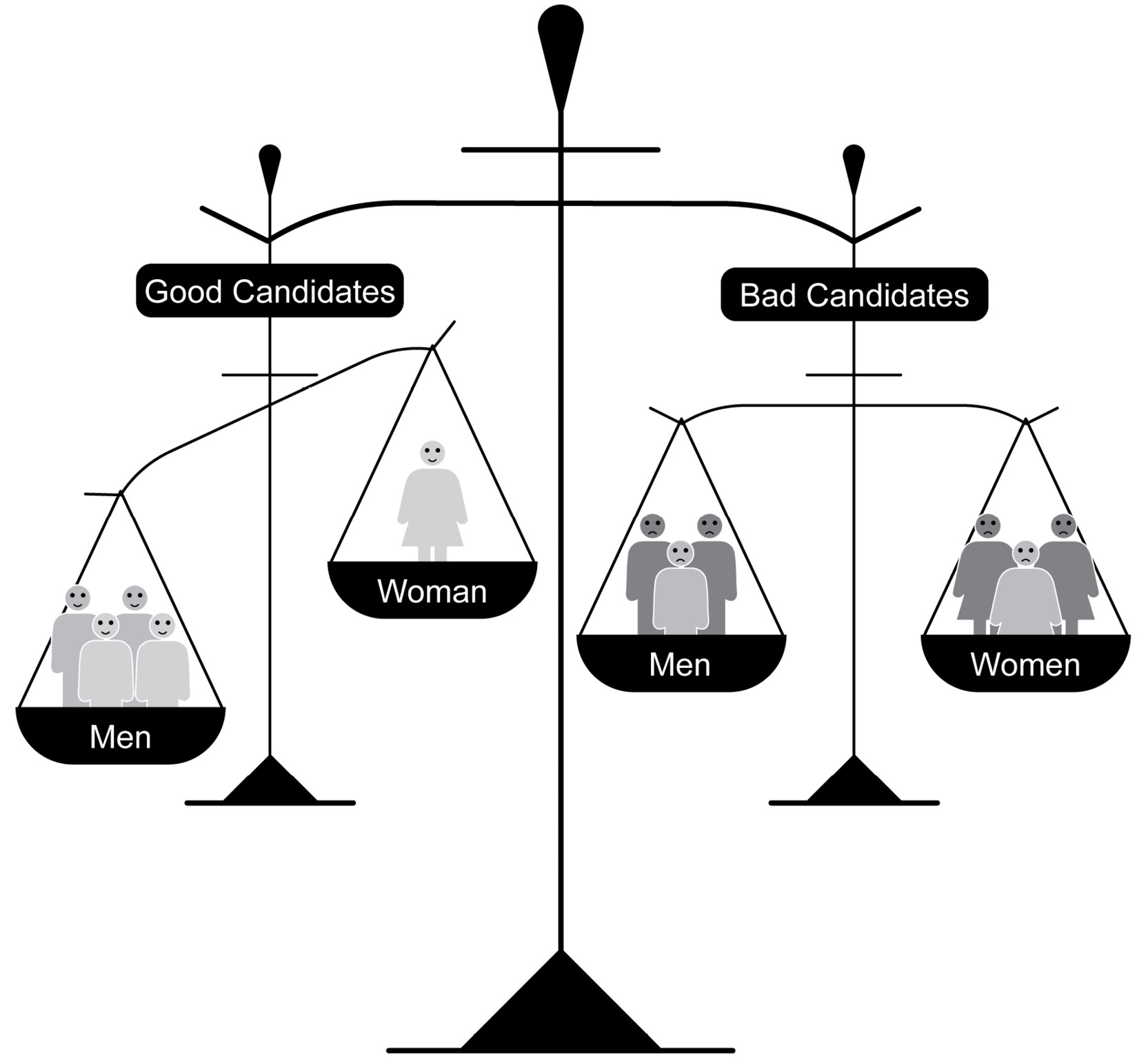
Figure 4.6: A partially balanced dataset – the quality of candidates is balanced,but gender is not balanced within the "good" class
Overall, the dataset was balanced, but there were more men in the "good candidates" class. As we already know, 80% of the "good" resumes are from male engineers while 20% are from female engineers who are working in Amazon. On the contrary, there was a more equal distribution in the "bad applicants" class.
If we explicitly use gender as one of the dimensions, the algorithm will quickly learn to favor male applicants, reinforcing biases that already plague Amazon's workforce.
It is unlikely that Amazon's algorithm would have explicitly used gender as an attribute to use in resume classification, but unfortunately, that does not stop a shrewd AI from picking up on the existing bias. For example, the resumes of many rejected candidates might have contained phrases such as "Women's chess club captain," or "Women's hockey coach," leading Amazon's algorithm to unfairly associate these words with bad candidates. On the other hand, men statistically use words such as "executed" and "captured" more often on their resumes, leading Amazon's algorithm to unfairly prefer candidates who use these words.
By internal accounts, phrases such as "Women's Chess Club Captain" were taken as a negative indicator, while words such as "executed" and "captured," which are found more often on men's resumes, were taken as positive.
No one explicitly asked the algorithm to do this, but they asked the algorithm to follow an example set by humans, and unfortunately, that example is often flawed.
In the previous case, there was a strong pattern, by many accounts, of Facebook and Cambridge Analytica claiming that they had not done anything wrong and refusing to accept accountability.
In this case, Amazon saw the problem and pulled the AI system at an experimental stage, before it could cause any harm in the real world, and this is already a key learning point for this.
Summary and Takeaways
In Chapter 1, Data Storage Fundamentals, we saw how good AI was at performing classification tasks—sorting data into two or more classes based on a deep analysis of many attributes. This works great for things such as spam classification and detecting cancer in X-rays, but can we use it to classify people? We can, but it's ethically very problematic. The way AI performs classification is by looking to exploit any bias in the data that it can, and many times the data is already affected by human biases, which AI is all too ready to take advantage of and reinforce.
Before building an AI system, we should ask whether it might be susceptible to bias through the following:
- Imbalances in the training dataset
- Existing human biases in the dataset
And we should also be wary of variables being modeled "by proxy." Sometimes, we do not want the algorithm to use specific aspects of the data such as gender, and so we remove it. However, it might still be possible for the algorithm to recalculate the missing pieces, based on what we left.
In the next case study, we will look at how AI is used in criminal justice.
Case Study 3: COMPAS Software
We have now seen two different ways that AI can cause harm if ethics is not considered. In the Cambridge Analytica case, the harm was abstract. No one was directly harmed, but we could argue that its results were a global harm through damage to our political systems.
In the second case, we saw that Amazon's hiring algorithm could have hurt people more directly: by rejecting them unfairly for jobs. But some people still might argue that this is not harmful enough to be worried. Some might argue that sexism is something that is a human problem and that the reinforcement of this is the price to pay for the benefits brought through AI efficiency.
In this case, we'll see how AI can cause direct and long-lasting harm to specific individuals by keeping them in prison. Being rejected from a job based on who you are is a terrible thing, but hopefully, you will be able to find another job. If you are kept in prison unfairly for 20 years, there is barely any compensation that can make up for that.
The US government uses predictive algorithms to decide who to keep in prison. These are based on trying to predict a criminal who might commit crimes again. It makes sense that we don't want to let people out of prison if they are likely to re-offend. But ethical considerations get complicated when we get a computer to help us make that decision.
The Correctional Offender Management Profiling for Alternative Sanctions(COMPAS) software used within the US judicial system is an example of exactly this. You give it all the details of a specific prisoner, and it spits out how likely that prisoner is to re-offend. It is not clear whether race is explicitly given as a variable to the COMPAS system, but this does not affect the result. As we saw in the case of Amazon, variables can be modeled by proxy. These are known as latent variables. For example, by looking at a combination of where a prisoner is originally from, who their relatives are, and which area they live in, the algorithm might be able to infer the prisoner's race. And, again, as we saw with the Amazon case, if a bias already exists in society, the algorithm could reinforce this bias.
The creators of COMPAS did try to control this in their software, and it seemed to predict equally that black and white defendants are likely to re-offend. At first glance, then, it looks like the algorithm has no racial prejudice. However, looking retrospectively at when the algorithm makes mistakes reveals a very different picture.
Classification algorithms can be wrong in two ways: they can have "false positives" and "false negatives." In COMPAS's case, they would be as follows:
- False positive: Predict that someone will re-offend, but they don't
- False negative: Predict that someone won't re-offend, but they do
Both cases are bad. In the first case, you keep someone in prison who shouldn't be there, and in the second case, you let someone out of prison who causes further harm to society:

Figure 4.7: COMPAS predictions representation
Even though COMPAS predictions on who will re-offend are split equally between black and white prisoners, it predicts almost twice as many false positives for black prisoners than for white prisoners. Furthermore, it predicts almost twice as many false negatives for white prisoners than for black prisoners.
This means that the algorithm often recommends keeping low-risk black defendants behind bars, and often recommends that high-risk white defendants should be released. It is acceptable and expected that the algorithm will sometimes make mistakes. However, it is hugely problematic to continue using software for something as important as keeping people in prison if it allows miscarriage of justice. This is especially true if it appears that this miscarriage happens through racism.
Summary and Takeaways
Using biased algorithms to assess who should be kept in prison has the potential to cause (and quite possibly does cause) concrete and direct ethical harm. This is in contrast to algorithms that violate privacy, which cause harm on a more abstract level.
We have seen how AI can cause harm intentionally or unintentionally, and how existing human biases, along with imbalanced datasets, can contribute toward the latter.
In this case, we saw that the COMPAS algorithm specifically seemed to pass initial bias tests. However, with more time and with analysis from outside researchers, we noticed that a few points had not been initially considered, some of which are as follows:
- These tests were not deep enough. They looked only at summary statistics on when the algorithm made mistakes, but not at the details of these mistakes.
- It took time and expertise to expose the details around how false positives were biased against black people.
Even if the problem were now fixed, it would not be acceptable for the people who fell victim to the false positives in the interim, and it is unfortunately not clear whether COMPAS changed their algorithm to account for the research. If they did make changes, it is difficult to verify that these changes fixed the problem.
Next, let's look at some more practical examples of how bias can be found in machine learning models.
Finding Built-In Bias in Machine Learning Models
We've seen how large and complicated systems can create ethical harm, and we've seen a strong theme of prejudice. In 2017, Robyn Speer wrote the article "How to make a racist AI without really trying." In this article, Speer showed how word vectors, a form of vectorized text, could be combined with a basic sentiment classifier. In Speer's examples, phrases that should be evaluated with a similar sentiment such as "Mexican food" and "Italian food" are given very different sentiment ratings. Because the word vectors are built from large corpora of human-written text, there is a negative sentiment toward specific racial groups, and this is apparent even when looking at phrases concerning food instead of people.
Let's take a deeper look at how word vectors work.
While the TF-IDF vectors we looked at in Chapter 1, Data Storage Fundamentals, are one way to vectorize words, these are character-based vectors. Using that method, there is no relation between "cat" and "kitten," as the words look very different. Word embeddings rely on a more complicated algorithm to convert text into vectors, but it has some of the advantages of structures such as TF-IDF. Word embeddings are trained using huge amounts of text data, and they look at what words often occur in similar contexts. Each word is represented as a vector with n dimensions, which can be thought of as a point in multidimensional space.
Just as a vector [3,4] might represent a point in two-dimensional space along an x- and y-axis, a word represented by a vector with 96 dimensions can be thought of as a point in 96-dimensional space. The word "machine" might look as follows:

Figure 4.8: The word "machine" as a word vector
It's hard thinking in terms of multidimensional space but remember that many of the rules that apply in two-dimensional space are valid in 300-dimensional space too. A recent discovery was that words that are semantically similar to "cat" and "kitten" can be close to each other in our multi-dimensional space, while words that are not related will be far away.
We will use the spaCy library to easily convert words into word vector representations and analyze these words by looking at their distances from other words.
As a very brief introduction, we can see that word embeddings, which are used in spaCy's pretrained models, are very powerful out of the box. In the following example, we're loading spaCy and comparing a few words using the similarity function, which simply looks at how close together words are in the multi-dimensional vector space described previously:
```
>>> import spacy
>>> nlp = spacy.load("en_core_web_lg")
>>> nlp("cat").similarity(nlp("kitten"))
0.821555342995594
>>> nlp("cat").similarity(nlp("dog"))
0.8016854705531046
>>> nlp("cat").similarity(nlp("cow"))
0.4746069221481621
>>> nlp("cat").similarity(nlp("coffee"))
0.2722319630373339
```
Cat and kitten are 82% similar, while cat and dog are 80% similar. Remember, word embeddings are based on context, so cat and dog might have a higher similarity than expected simply because the two words are often used in the same context; for example, "yesterday I fed my dog" and "yesterday I fed my cat" are both valid and common sentences.
There is some similarity between "cat" and "cow" (they are both animals), but very little similarity between "cat" and "coffee."
Therefore, even without teaching a computer what "good" or "bad" are (or "positive" or "negative"), we can build a very basic sentiment classifier by seeing how close words and phrases are to "good" and "bad".
spaCy is useful because we can use it, as humans, to operate directly on strings such as "cat." Internally, spaCy will convert this into a vectorized representation that we can inspect by using the .vector attribute, as shown in the following figure:

Figure 4.9: Looking at the vector for "cat" using spaCy
We can even check the total vectors in which SpaCy has converted the string using the vector.size attribute, as shown in the following figure:
>>> nlp("cat").vector.size
300
Exercise 4.01: Observing Prejudices and Biases in Word Embeddings
In this exercise, we're going to build a prejudiced AI using sentiment analysis. You'll write some Python code, use the spaCy library, and get a hands-on feel for how word vectors (also known as word embeddings) work.
By the end of this exercise, you will have built a very crude form of sentiment classifier, but it will be enough to see some biases and prejudices that are to be expected whenever we start looking at large amounts of text data.
Before proceeding to the exercise, we need to install the spaCy library, along with large pre-trained models, in the local dev environment. Please follow the instructions in the Preface to install it.
Perform the following steps to complete this exercise:
- Create a directory called Chapter04 for all the exercises of this chapter. In the Chapter04 directory, create the Exercise04.01 directory to store the files for this exercise.
- Open your Terminal (macOS or Linux) or Command Prompt (Windows), navigate to the Chapter04 directory, and type jupyter notebook. The Jupyter Notebook should look as follows:
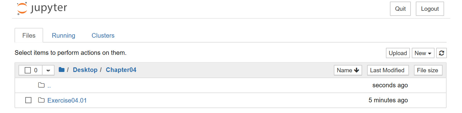
Figure 4.10: The Chapter04 directory in the Jupyter Notebook
- Select the Exercise04.01 directory and click New -> Python3 to create a new Python 3 notebook:
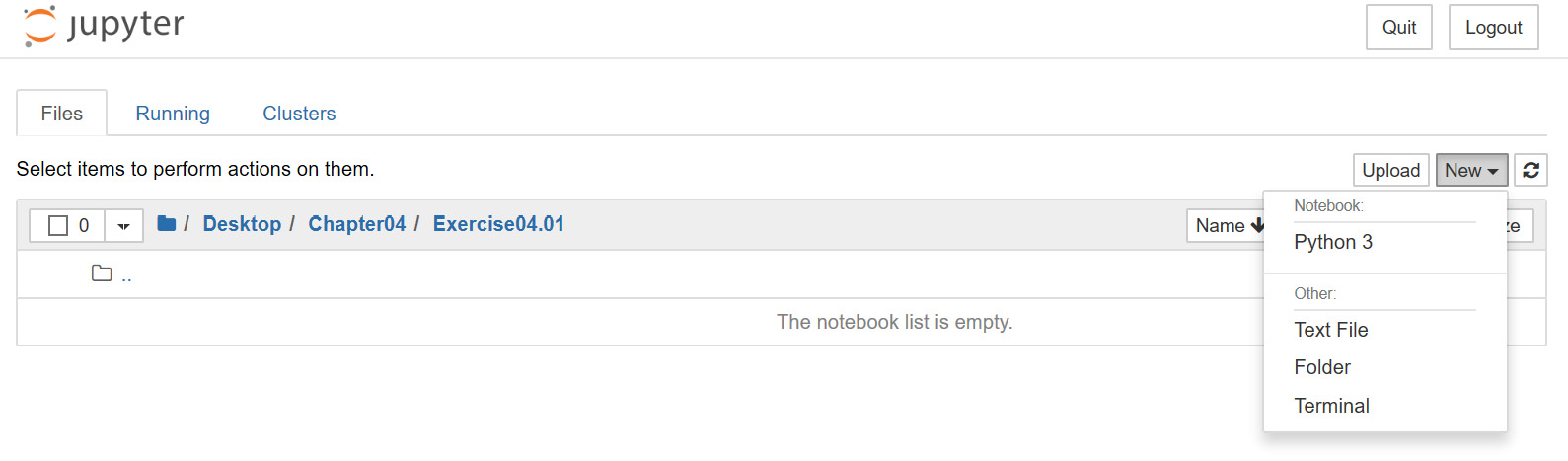
Figure 4.11: The Exercise04.02 directory in the Jupyter Notebook
- Import spaCy and load the pre-trained model:
import spacy
nlp = spacy.load('en_core_web_lg')
Note that the model file is large and that it will probably take quite a few seconds to run this, depending on your machine.
- Parse "good" and "bad" into variables to see how close other words are to them, as shown in the following code:
good = nlp("good")
bad = nlp("bad")
- Compare the word awful to the words good and bad, as shown in the following code:
print(nlp("awful").similarity(bad))
print(nlp("awful").similarity(good))
You should get the following output:
0.7721672894451931
0.551066389568291
The output shows that awful is 77% similar to bad and 55% similar to good. However, awful is fairly similar to both concepts, as it used in the same contexts. Let's try a more abstract concept: night and day. Traditionally, "day" is used in more positive settings (for example, "a new day") and night in more negative ones (for example, "For the night is dark and full of terrors").
- Compare day to good and bad, as shown in the following code:
print(nlp("day").similarity(bad))
print(nlp("day").similarity(good))
You should get the following output:
0.4455448306231779
0.5082143964475753
- Compare night to good and bad, as shown in the following code:
print(nlp("night").similarity(bad))
print(nlp("night").similarity(good))
You should get the following output:
0.45386439630840125
0.4425397729689741
Note that both words are less like both good and bad than the word awful. When we look at sentiment using this crude definition, we aren't interested in the absolute distances between these concepts, but rather we are interested in the relative distance. Is a particular word closer to good than it is to bad or vice versa? Let's define a basic function to allow us to calculate this.
- Define a polarity function to calculate whether a word is closer to good or closer to bad, as shown in the following code:
def polarity_good_vs_bad(word):
"""Returns a positive number if a word
is closer to good than it is to bad,
or a negative number if vice versa
IN: word (str): the word to compare
OUT: diff (float): positive if the word
is closer to good, otherwise negative
"""
good = nlp("good")
bad = nlp("bad")
word = nlp(word)
if word and word.vector_norm:
sim_good = word.similarity(good)
sim_bad = word.similarity(bad)
diff = sim_good - sim_bad
diff = round(diff * 100, 2)
return diff
else:
return None
The preceding code takes in a string (word) as an argument. It creates vector representations based on the pre-trained vectors that ship with spaCy for three words: good, bad, and the passed-in word. It then looks at the distance in vector space between that passed-in word and the good and bad vectors and calculates the difference between these. Therefore, a closer (more similar) word to good will have a positive value and a word that is closer (more similar) to bad will have a negative value.
Note that the differences are often quite small, so we multiply by 100 to magnify them and make them more interpretable to humans.
- Now, we need to create a function to display the polarity of words which have opposite meanings :
def contrast_pairs(pairs):
for pair in pairs:
pos_word = pair[0]
neg_word = pair[1]
pos_score = polarity_good_vs_bad(pos_word)
neg_score = polarity_good_vs_bad(neg_word)
print(f"{pos_word}({pos_score}):
{neg_word}({neg_score})")
- And now, we need to test our polarity function with words of opposite meanings:
word_pairs_neutral = [
('day', 'night'),
('light', 'dark'),
('happy', 'sad'),
('love', 'hate'),
('strong', 'weak'),
('healthy', 'sick'),
('free','captive'),
('high', 'low')
]
contrast_pairs(word_pairs_neutral)
You should get the following output:

Figure 4.12: Comparing the scores of positive and negative words
As expected, some opposites such as healthy and sick show a very strong difference in polarity, while others such as day and night or high and low are less obvious, but still have some sentiment attached to them. Let's see what happens if we look at word pairs that are more closely associated with current and historical prejudices.
- Compare polarity scores for words often associated with prejudice, as shown in the following code:
word_pairs_prejudice = [('white', 'black'),
('christian', 'jew'), ('christian', 'muslim'),
('christian', 'atheist'), ('man', 'woman'),
('king', 'queen'), ('citizen', 'immigrant'),
('resident', 'migrant'), ('rich', 'poor'),
('engineer', 'janitor'), ('young', 'old'),
('pizza', 'sprout'), ('native', 'foreigner'),
('italian', 'iranian'), ('swiss', 'mexican'),
]
contrast_pairs(word_pairs_prejudice)
- You should get the following output:
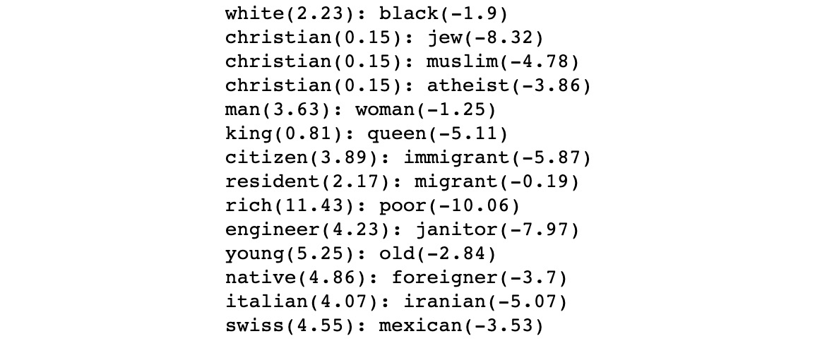
Figure 4.13: Comparison of scores for word pairs associated with prejudices
Note
To access the source code for this specific section, please refer to https://packt.live/3elL7Ch.
While this is a small set of examples and does not prove anything, we can see that there is likely some kind of latent prejudice in our pre-trained model. We can see some strong elements of sexism (man is better than the woman), racism (white is better than black), classism (rich is better than poor), and religious prejudice (Christian is better than jew, Muslim, and atheist).
Remember that the word vectors are created by using large amounts of human-created training data. Although spaCy changes the data sources from time to time, in the examples shown here, we used the default built-in spaCy model, which is trained on the OntoNotes dataset. This is a collection built from telephone conversations, newswire, newsgroups, broadcast news, broadcast conversation, and weblogs, and we can easily imagine how existing human prejudices might be represented in these datasets.
With that, we have seen how our sentiment classifier performed in this toy example, where we made up some data. We'll try it with a proper dataset in the next exercise.
Exercise 4.02: Testing Our Sentiment Classifier on Movie Reviews
Sentiment analysis is a huge field on its own, and it is actively evolving. There are many very sophisticated sentiment models, but the one we built in the previous exercise is very crude indeed. In this exercise, we'll see how the classifier performs on the common task of discriminating between movie reviews. Reviewers leave positive or negative text associated with a star rating between 1 and 10 on internet sites such as IMDb. If our algorithm knows what kind of words are "good" and which ones are "bad," it should be able to tell the difference between good and bad movie reviews without using the star rating.
We'll use the aclImdb dataset of 100k movie reviews from IMDb, 50k each for training and testing. Each dataset has 25k positive reviews and 25k negative ones, so this is a larger dataset than our headlines one. The dataset can be found in our GitHub repository at the following location: https://packt.live/2C72sBN.
You need to download the aclImdb folder from the GitHub repository.
Dataset Citation: Andrew L. Maas, Raymond E. Daly, Peter T. Pham, Dan Huang, Andrew Y. Ng, and Christopher Potts. (2011). Learning Word Vectors for Sentiment Analysis. The 49th Annual Meeting of the Association for Computational Linguistics (ACL 2011).
Perform the following steps to complete this exercise:
- Create the Data and Exercise04.02 directories in the Chapter04 directory to store the files for this exercise.
- Move the aclImdb folder to the Data directory.
- Open your Terminal (macOS or Linux) or Command Prompt (Windows), navigate to the Chapter04 directory, and type jupyter notebook.
- In the Jupyter Notebook, click the Exercise04.02 directory and create a new notebook file with the Python3 kernel.
- Import the same libraries as before, along with matplotlib, so that we can do some plotting, as shown in the following code:
%matplotlib inline
import spacy
import os
import numpy
from matplotlib import pyplot as plt
from statistics import mean, median
In this code, we imported the libraries that we need. Note that we use %matplotlib inline right at the top of the notebook file to make our plots display correctly.
- Load spacy and define our polarity function, as shown in the following code:
nlp = spacy.load('en_core_web_lg')
def polarity_good_vs_bad(word):
"""Returns a positive number if a word
is closer to good then it is too bad,
or a negative number if vice versa
IN: word (str): the word to compare
OUT: diff (float): positive if the
word is closer to good, otherwise negative
"""
good = nlp("good")
bad = nlp("bad")
word = nlp(word)
if word and word.vector_norm:
sim_good = word.similarity(good)
sim_bad = word.similarity(bad)
diff = sim_good - sim_bad
diff = round(diff * 100, 2)
return diff
else:
return None
As in the previous exercise, the preceding code takes in a string (word) as an argument. It creates vector representations based on the pre-trained vectors that ship with spaCy for three words: good, bad, and the passed-in word. It then looks at the distance in vector space between the passed-in word and the good and bad vectors and calculates the difference between them. Therefore, a closer (more similar) word to good will have a positive value and a word that is closer (more similar) to bad will have a negative value.
- Now, loop through each review in the pos and neg subdirectories of the train folder and calculate the sentiment score for each, keeping two distinct arrays of positive and negative reviews:
Note
Make sure you change the path to the train folder based on its location on your system.
review_dataset_dir = "../Data/aclImdb/train"
pos_scores = []
neg_scores = []
LIMIT = 2000
for pol in ("pos", "neg"):
review_files = os.listdir(os.path.join(
review_dataset_dir, pol))
review_files = review_files[:LIMIT]
print("Processing {} review files"
.format(len(review_files)))
for i, rf in enumerate(review_files):
with open(os.path.join(review_dataset_dir,
os.path.join(pol,rf)), encoding ="utf-8") as f:
s = f.read()
score = polarity_good_vs_bad(s)
if pol == "pos":
pos_scores.append(score)
elif pol == "neg":
neg_scores.append(score)
You should get the following output:
Processing 2000 review files
Processing 2000 review files
We grabbed some files from each of the neg (negative) and pos (positive) training folders, calculated the polarity score for each using our crude sentiment analyzer from Exercise 4.01, Observing Prejudices and Biases in Word Embeddings, and keep a record of these scores. If the sentiment analyzer is good, it will give high scores to the pos reviews and low scores to the neg reviews.
- Calculate the mean and median of each set of scores:
mean_pos = mean(pos_scores)
mean_neg = mean(neg_scores)
med_pos = median(pos_scores)
med_neg = median(neg_scores)
print(f"Mean polarity score of positive reviews:
{mean_pos}")
print(f"Mean polarity score of negative reviews:
{mean_neg}")
print(f"Median polarity score of positive reviews:
{med_pos}")
print(f"Median polarity score of negative reviews:
{med_neg}")
You should get the following output:
Mean polarity score of positive reviews: 4.88497
Mean polarity score of negative reviews: 3.220575
Median polarity score of positive reviews: 4.84
Median polarity score of negative reviews: 3.29
We can see that there is some difference in the direction that we expect, with the positive reviews, on average, having a higher polarity score than the negative ones.
Note that we used two average functions: mean and median. The median is a useful average when you expect some outliers in your distribution to have undue influence. In our case, the two averages are quite similar, so there are probably not many outliers. Interestingly, the negative reviews have an on-average positive polarity score. Let's look at the distribution of both classes.
- Plot histograms of the scores for positive and negative reviews:
bins = numpy.linspace(-10.0, 10.0, 50)
plt.hist(pos_scores, bins, alpha=0.9, label='pos')
plt.hist(neg_scores, bins, alpha=0.9, label='neg')
plt.legend(loc='upper right')
plt.show()
You should get the following output:
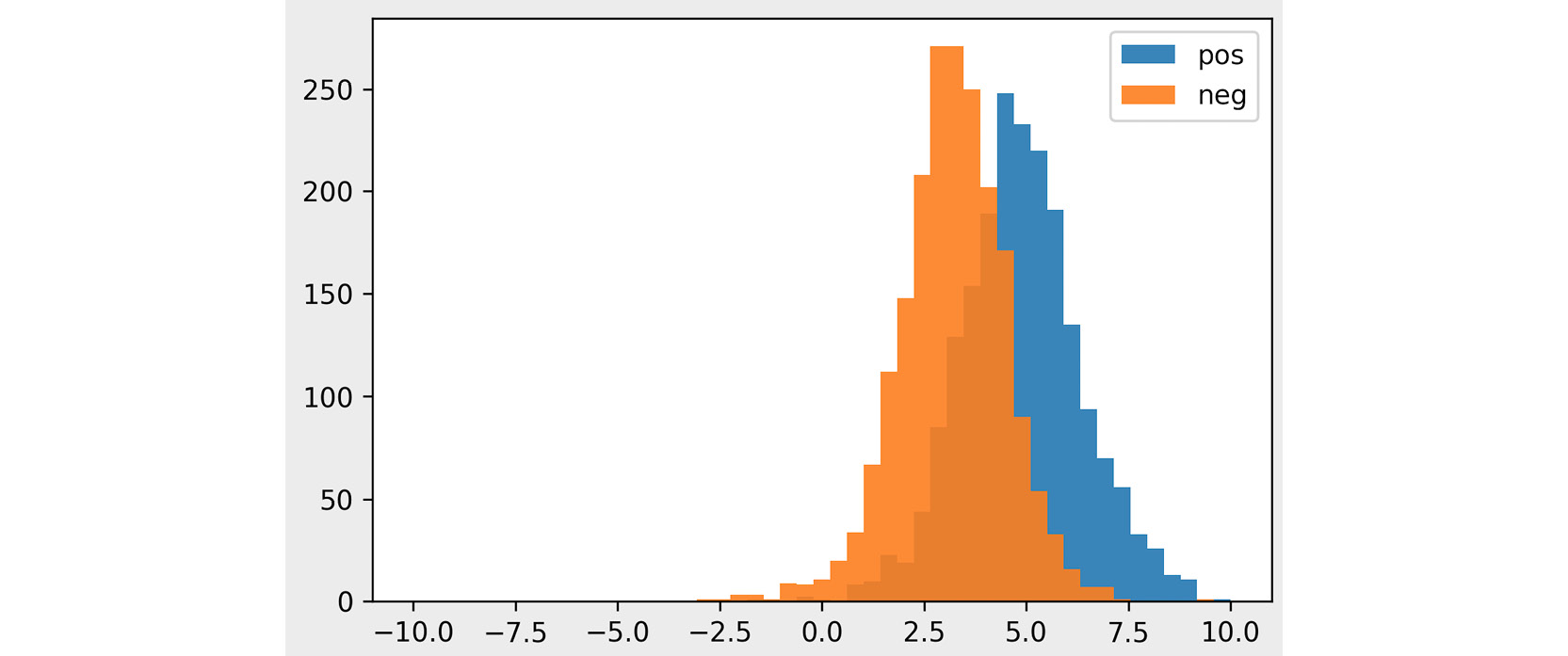
Figure 4.14: The distribution of polarity scores for positive and negative movie reviews
The preceding chart shows a histogram of polarity scores for positive and negative reviews. The x-axis shows the polarity scores, while the y-axis shows the number of reviews with that score. For example, we can see that over 250 negative reviews have a polarity score of 2.5, while only about 50 positive reviews have this score. The range of polarity scores is between -10 and 10, with nearly all reviews falling between -1 and 9. These exact numbers don't mean anything on their own, but they show us relatively well which reviews are regarded as more positive.
We can see that the trend is in the right direction but that the scores are not enough to fully differentiate between positive and negative movie reviews. One important limitation of our classifier is that it is based on single words and not phrases. Language is complicated. Let's look at how words such as "not" can make sentiment analysis more difficult.
- Calculate the polarity scores of some phrases relating to how good or bad a movie was:
phrases = [
"the movie was good",
"the movie was not good",
"good",
"not",
"the movie was very good",
"the movie was very very good",
"the movie was bad",
"the movie was very very very bad"
]
for phrase in phrases:
print(phrase, polarity_good_vs_bad(phrase))
You should get the following output:

Figure 4.15: The polarity scores of short, invented move reviews
Because our crude polarity calculator averages together the "meanings" of words by using their word vectors, the phrase not good is the average of the words not and good. Now, Good has a strongly positive score, and not has a neutral score, so not good is still seen as positive overall. On the other hand, very is closer to good in our vector space than it is to bad, so with enough occurrences of very in a phrase, the negative score from bad can be canceled out, leaving us with an overall positive score.
Note
To access the source code for this specific section, please refer to https://packt.live/38QwJAV.
In this exercise, we built a polarity classifier. We fed movie reviews into it and we saw that it worked as expected. On average, it gave higher scores for positive movie reviews and lower scores for negative movie reviews. The fact that we can verify that our classifier does work for a normal sentiment classifier task makes it more concerning that it displays some prejudices.
In the next activity, you will use the classifier for a third time and see what other prejudices it might display.
Activity 4.01: Finding More Latent Prejudices
Imagine that you have built the preceding classifier and have noted potential ethical concerns. You need to further validate your assumption that the model displays problematic prejudices.
You aim to further test the classifier with a wider range of inputs and to see whether you can predict what it will output.
You should build your word list of concepts that might have a prejudiced association and try to predict whether the classifier will classify them as positive or negative. You should then test your assumptions by running the words through the classifier.
Note
The code and the resulting output for this exercise have been loaded into a Jupyter Notebook that can be found here: https://packt.live/2OxwZeZ.
Perform the following steps to complete this activity:
- Create a list of at least 16 words that you think might have a positive or negative prejudice. We are using the following 16 words for this activity:
sporty
nerdy
employed
unemployed
clever
stupid
latino
asian
caucasian
disabled
pregnant
introvert
extrovert
politician
florist
- Define the same classification model that we used in previous exercises.
- Before running the code, guess whether each of the words you chose would be classified as a positive or negative word. We have guessed the words (sporty, employed, clever, caucasian, extrovert, and florist) as positive and the remaining ones as negative.
- Run the classifier on the word list and see how close your predictions were.
You should get the following output:

Figure 4.16: The polarity scores for each word in our new list
In our activity, we gained further evidence that our classifier might display prejudices. Let's move on and close this chapter.
Note
The solution to this activity can be found on page 595.
Summary
In this chapter, we saw examples of prejudice in AI systems through several case studies. We saw how Cambridge Analytica developed an AI based on stolen personal data, how Amazon developed an AI that displayed sexist traits, and how the US justice system, to some extent, relies on AI that displays racist traits.
We built our own AI system that displayed some elements of prejudice and discussed how important it is to be aware of in-built biases, especially when using pre-trained models. We gained experience with the Python library spaCy and saw how word embeddings work. We verified that our sentiment analyzer worked on movie reviews, and then tested it further with some more words associated with prejudices.
In the next chapter, we will be studying the fundamentals of SQL and NoSQL databases by taking a practical approach. We will be learning and performing queries in MySQL, MongoDB, and Cassandra. Don't forget to consider the ethical considerations of any data that you store.