5. Data Stores: SQL and NoSQL Databases

Overview

In this chapter, we will study the SQL and NoSQL databases. First, you will learn how to decide on the ideal database to be used based on the format of the data at hand. Then, we will implement storing and querying data in different databases such as MySQL, MongoDB, and Cassandra. Furthermore, to improve efficiency, we will optimize the databases for maximum performance. This chapter includes hands-on experiences so that you can learn how to deal with practical real-world problems related to databases. By the end of this chapter, you will be able to develop and implement data models on MySQL, MongoDB, and Cassandra databases.

Introduction

In the previous chapter, we covered case studies on how AI has been controversial, along with various industry-standard use cases and hands-on information about the tools and frameworks related to storage. In a continuation of earlier discussions, we will be diving into detailed discussions on the kinds of databases that are available, along with their evolution, internal structures, and best possible use cases and examples.

Understanding database management is quite important as it gives you a clear idea about how data flows, that is, the transaction of data between the application and the database. For businesses and organizations, multiple types of data can be handled quite effectively using the knowledge of database management. Nevertheless, there are several challenges associated with data storage, such as infrastructure, cost, compatibility, and security.

In practical scenarios, databases enable us to accelerate our predictive analytics power by deploying Artificial Intelligence (AI) to get rid of several real-world problems such as credit card fraud detection, stock market prediction, and early stage disease detection.

Currently, various kinds of databases are available on the market, such as Relational (SQL), Document store (MongoDB), Columnar (Cassandra), Key-Value store (NoSQL), and Graph (ArangoDB) databases. Each of these databases has its characteristics and advantages and disadvantages. These databases are broadly divided into two groups: SQL and NoSQL databases.

SQL databases are relational database systems (RDBMS), which are structured/relational databases. The main language that's used to deal with the data is Structured Query Language (SQL). It is used to form a query and access the data.

NoSQL databases are Not Only SQL databases, wherein the data is in a semi-structured format. The main language that deals with data can vary for each database. This type of database has triggered the evolution of large distributed data stores running over a bunch of commodity hardware called nodes. Without the ability to use distributed data stores and having our data stored on a cluster of inexpensive nodes, we would have to rely on expensive single machines with very large capacities. This is not only expensive, but it also presents a single point of failure infrastructure. Generally, these databases are used where the data is huge and needs to be accessed at the lowest latency possible.

In this chapter, we are going to learn about the relational, document store, and columnar databases by going through examples and case studies. Lastly, we will learn how these databases are used in a hybrid architecture. In the next section, we will discuss database components to understand concepts including the query engine and interface, tables, schemas, and buffer pool.

Database Components

The typical database components can be seen in the following diagram. These components include the following:

• Query Engine & Interface: A translation unit that translates the query into a machine-readable language.
• Tables: Collection of rows where the actual data is stored. Tables can be accessed via the query engine.
• Schemas: Collection of tables where each schema represents a functional group of tables; for example, HR and Payroll.
• Buffer pool: A component that holds recent or intermediate transaction data in memory for optimized operation execution:
  

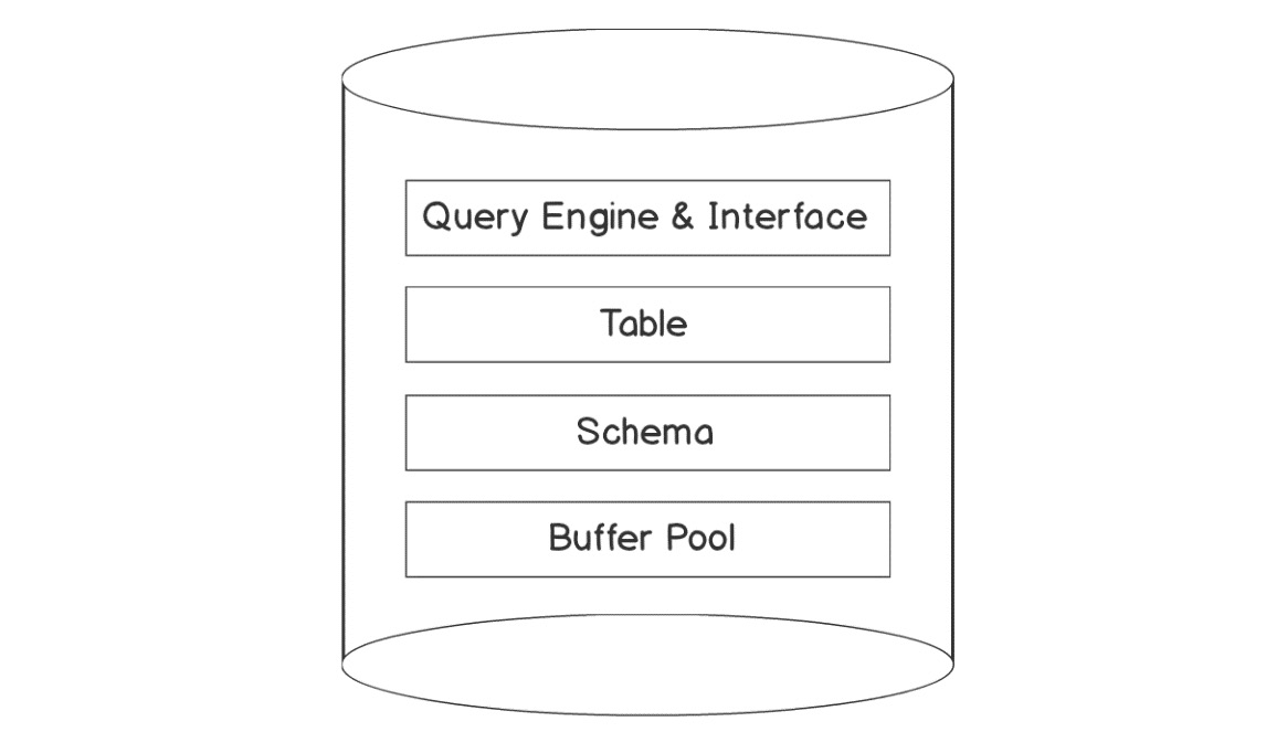
Figure 5.1: Typical database components

SQL Databases

These are the row-oriented type of databases. Here, each row of the database is a record. A collection of columns forms a record and is stored in a structure called a table. These collections of tables form the database.

These databases are accessed using SQL. It was developed by two IBM software researchers in the 1970s and it became more and more dominant in the field after that due to its straightforward, understandable syntax, ease of learning, and fewer lines of code being required to use complex functionalities:

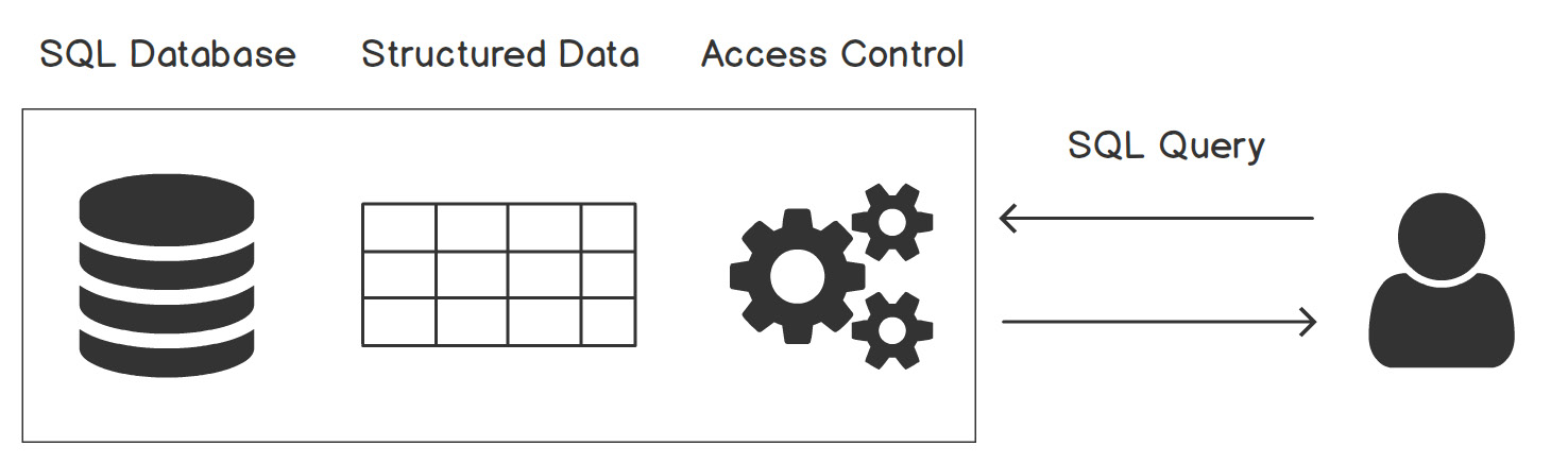
Figure 5.2: User database interaction through SQL

In the preceding diagram, user database interaction through SQL is demonstrated, where the efficacy of the SQL architecture to deal with "structured data" is quite visible.

SQL databases work on Atomicity, Consistency, Isolation, and Durability (ACID) properties, which guarantees strong consistencies and isolated transaction behavior. These are crucial while designing a data storage system.

Also, when we think about AI, having just one type of database is not sufficient due to the various forms of data. Therefore, there is a need for a hybrid data architecture in various cases, as we covered in the last section, Exploring the Collective Knowledge of Databases, of the chapter. In some hybrid architectures, we use the properties of the consistency and availability of MySQL and Mongo DB, respectively.

Undoubtedly, MySQL and Oracle are the most popular choices among RDBMS, as per their efficacies, but we will restrict our discussions to just MySQL in the next section as it is open source.

MySQL

MySQL is an open source relational database system that's used by websites such as Facebook, Flickr, Twitter, and YouTube because it supports stored procedures, cursors, triggers, and all the SQL database features.

Advantages of MySQL

• Simple and easy to use
• Open-source
• Good performance with a wide range of queries and primary keys
• Effectively processes data that's GBs to a few TBs in size, with a limited level schema complexity
• Follows the ACID methodology accurately
• Follows the schema-on-write methodology where it pre-validates the records during insertion

Disadvantages of MySQL

• Difficult to scale MySQL after a certain level.
• Designed to run on a single machine, which means a single point of failure and lesser availability.
• Being a part of the relational database system focuses on normalization and data duplication, which results in multiple joins. After a while, when data grows exponentially, this leads to a massive problem, especially for use cases such as user activity logging.
• Not appropriate in the case of read-heavy systems with high complexity schemas.

Query Language

As you already know, MySQL uses the SQL language to deal with data. Let's take a look at the syntax and semantics.

Terminology

SQL is a structured query language; it is composed of predicates or clauses:

• A column is a single field in the data; it's a single unit of data.
• A row is a collection of columns.
• A table is a collection of rows.
• A database is the collection of tables.

Data Definition Language (DDL)

The following SQL commands are used to deal with the structure of the database or table:

• CREATE DATABASE

  This command creates a database:

  CREATE DATABASE fashionmart;

• CREATE TABLE

  This clause is used to create a table. Here, you have to specify the columns and their data types and constraints:

  CREATE TABLE products (p_id INT,

                         p_name TEXT,

                         p_buy_price FLOAT,

                         p_manufacturer TEXT,

                         p_created_at TIMESTAMP,

                         PRIMARY KEY (p_id)

                         );

  This command will create a table product that has five columns. p_id will have PRIMARY KEY as a constraint. We will discuss the primary key later.

• DESC

  The table structure can be displayed using this command:

  DESC products;

• ALTER TABLE

  This clause is used to modify the table structure to, for example, add, rename, or drop a column:

  ALTER TABLE products ADD COLUMN p_modified_at TIMESTAMP NOT NULL;

  Note

  In case you run into an error while running the preceding code, you can set the SQL_MODE in MYSQL to Allow Invalid Dates using the following command: SET SQL_MODE='ALLOW_INVALID_DATES';

  In this command, we have added the p_modified_at column with the TIMESTAMP data type and the NOT NULL constraint.

• DROP TABLE

  This command drops the table and removes all the records:

  DROP TABLE products;

Data Manipulation Language (DML)

The following SQL commands are used to deal with the actual data in the table:

• INSERT

  This command is used to insert records into the table:

  INSERT INTO products (p_id, p_name, p_buy_price,

                        p_manufacturer, p_created_at)

  VALUES (1, 'Z-1 Running shoe', 34, 'Z-1', now());

  In this command, columns can be specified after the table name and the values inside the VALUES clause.

  Adding single rows for multiple queries is exhausting and time-consuming. We can add multiple rows in a single query like so:

  INSERT INTO products(p_id, p_name, p_buy_price,

                       p_manufacturer, p_created_at)

  VALUES

  (2, 'XIMO Trek shirt', 15, 'XIMO', now()),

  (3, 'XIMO Trek shorts', 18, 'XIMO', now()),

  (4, 'NY cap', 18, 'NY', now());

• UPDATE

  This command is used to update existing records inside the table:

  UPDATE products SET p_buy_price=40

  WHERE p_id=1;

  In this command, the SET clause is used to set a value for the column, while the WHERE clause filters the rows for the matching condition. If the condition is missing, it will update the value for all the records. In this example, we are updating the buy price to 40 for the product whose ID is 1 in the products table.

• DELETE

  This command is used to delete records from the table:

  DELETE FROM products WHERE p_id=1;

  Here, if the condition is not given, then it will delete all the records from the table. As we have given the condition where the product ID is 1, it will only delete that record.

Data Control Language (DCL)

The following SQL commands are used to deal with providing control access to data stored in a database:

• GRANT

  This command allows the owner of the object with GRANT access to accord privileges to other users. The syntax for the GRANT command is as follows:

  GRANT privilege_name ON object_name

  TO {user_name | PUBLIC | role_name} [with GRANT option];

  An example of the GRANT command is as follows:

  GRANT SELECT ON student TO user5

  This command grants a SELECT permission on the student table to user5.

• REVOKE

  This command cancels previously granted or denied permissions. The syntax for the REVOKE command is as follows:

  REVOKE privilege_name ON object_name

  FROM {User_name | PUBLIC | Role_name}

  An example of the REVOKE command is as follows:

  REVOKE SELECT ON student TO user5

  This command revokes the SELECT permission on the student table from user5.

Transaction Control Language (TCL)

The following SQL commands are used to deal with SQL's logical transactions:

• COMMIT

  This command permanently saves any transaction in the database. The syntax is as follows:

  COMMIT;  

• ROLLBACK

  This command restores the database to the last committed state. The syntax is as follows:

  ROLLBACK;

• SAVEPOINT

  This command temporarily saves a transaction so that we can roll back to that point if required. The syntax is as follows:

  SAVEPOINT savepoint_name;

To retrieve data in SQL, we often use the SELECT statement as it plays a significant role. Now, let's discuss data retrieval in terms of the appropriate commands and examples of how to use them.

Data Retrieval

This section focuses on data access:

• SELECT

  This command is used to access the data from the table:

  SELECT * FROM products;

  This command will display all the records from the products table. Here, the FROM clause specifies the table name.

• JOINS

  To compare and combine in SQL, joins are used. As output joins return specific rows of data from two or more tables in a database. Hence, this is not a command but a concept, where we can join more than one condition based on another condition. Let's understand this better by going through an example. Consider we have two tables, sales, and products, with the following data:

  

Figure 5.3: Data of the sales and products tables

Using the following code, we will join the sales table with p_id as the FOREIGN KEY pointing to the products table:

SELECT

  products.p_name AS product_name,

  products.p_manufacturer AS manufacturer,

  sales.s_profit AS profit

FROM products

JOIN sales

ON products.p_id=sales.p_id;

This should give us the following output:

Figure 5.4: Joined data on the sales and products tables

This command joins products and sales using the JOIN and ON clauses. The ON clause holds the condition to join.

There are various types of joins available. The one we observed in the previous example was an inner join. Conceptually, inner joins find and return matching data from tables, whereas outer joins find and return matching data, as well as some dissimilar data from tables. Let's discuss outer joins by going through several examples.

LEFT OUTER JOINS

This join, in the preceding scenario, will show non-matching data from the left table, products; that is, data from the products table that does not have sales data associated with it:

SELECT

  products.p_name AS product_name,

  products.p_manufacturer AS manufacturer,

  sales.s_profit AS profit

FROM products

LEFT OUTER JOIN sales

ON products.p_id=sales.p_id;

This should give us the following output:

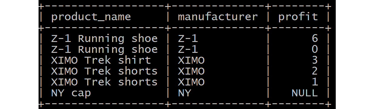
Figure 5.5: Left outer join over the sales and product tables

RIGHT OUTER JOINS

This join, in alternate scenarios, will show non-matching data from the right table, sales; that is, data from the sales table that does not have products table data associated with it:

SELECT

  products.p_name AS product_name,

  products.p_manufacturer AS manufacturer,

  sales.s_profit AS profit

FROM products

RIGHT OUTER JOIN sales

ON products.p_id=sales.p_id;

This should give us the following output:

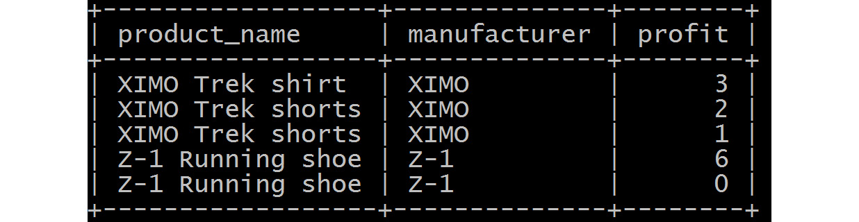
Figure 5.6: Right outer join over the sales and product tables

• Aggregate functions and GROUP BY

  The GROUP BY clause is used to group records on one or more columns and then perform all the operations associated with it. One thing to take care of is that the column not used in aggregate functions should be included in the GROUP BY clause.

  Aggregate functions include SUM, MIN, MAX, COUNT, and AVG. Let's look at an example:

  SELECT

    sales.p_id AS p_id,

    SUM(sales.s_profit) AS profit

  FROM sales

  GROUP BY sales.p_id;

  This command is grouping the table on the p_id column and performing addition (using the SUM function) over the profit column to find out the total profit for each p_id. You can use any aggregate function with the GROUP BY clause.

  This should give us the following output:

  

Figure 5.7: SUM (Aggregate) function over profit in the sales table

• ORDER BY

  This clause is used to sort the result on a column. ORDER BY executes last in query lineage. You can sort the column in ascending or descending order:

  SELECT

    sales.p_id AS p_id,

    SUM(sales.s_profit) AS profit

  FROM sales

  GROUP BY sales.p_id

  ORDER BY profit ASC;

  This should give us the following output:

  

Figure 5.8: SUM (aggregate) function over profit in the sales table, ordered by profit

SQL Constraints

This section is dedicated to the constraints/rules in the table. These constraints help MySQL pre-validate the record before inserting it into the table. These constraints can be created by using the CREATE TABLE statement. We will discuss a few constraints here.

The following are the main constraints:

• PRIMARY KEY: This specifies the main ID column of the table. This should be unique and not null.
• FOREIGN KEY: This allows us to ensure the referential integrity of data. This specifies the relationship between two tables. While declaring it, you can use ON DELETE CASCADE, which implies that if the parent data is deleted, the child data record is automatically deleted.
• UNIQUE: This constraint specifies that non-duplicate records are accepted.
• NOT NULL: This constraint specifies that any value of the column should not be null.

To understand the importance of SQL databases, let's take an example of a store called FashionMart that sells products such as clothing and jewelry to its customers. We have been given the task of making an online e-commerce website for the store. Initially, we want to achieve the following tasks with this website:

• Store the product information in the inventory
• Store the selling prices and calculate profits

Let's assume that we saved this information in file storage such as Products.csv and Sales.csv files. Now, we can easily add a new product to Products.csv and also add new sales data to Sales.csv; all you need to do is append one record to the end of the file:

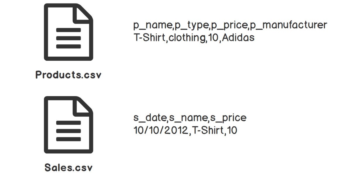
Figure 5.9: Products and sales data representation in the file

At this point, everything is working fine, but suddenly, the store owner finds out that one of the product's prices and names needs to be changed. So, to apply these changes, the product entry record needs to be found in Products.csv and then modified. Even after doing this, there will be records with duplicate product names in Sales.csv that need to be changed. This will lead to inconsistency in the data and its management becoming tedious. So, it's clear that file storage is not a good option for this use case. There are some more points to consider, such as a lock on the file when the file is being read/modified simultaneously. Also, if there are a million products in the store, how efficient will the search be?

Considering the previous criteria, we need to build the data system so that users can digitally run the FashionMart store. The following exercise focuses on designing a data model for the database and converts this CSV-based non-maintainable data system into a relational database system.

Let's design a basic building block of the database, that is, a data model.

A data model is a way of representing entities and their inter-relationships. We will discuss data modeling in detail later in this chapter:

Figure 5.10: Data model for FashionMart

This data model gives us an overview of a relational database consisting of two tables, Products, and Sales. Products contains fields such as p_id, p_name, p_buy_price, p_manufacturer (we could also have a manufacturer table and refer to it here with a foreign key), and p_created_at, while the Sales table has fields such as s_id, p_id (foreign key of the Products table), s_sale_price, s_profit, and s_created_at. This data model prevents the duplicity of product name data and overcomes problems we saw in the file storage system.

Since the physical data model is ready, we'll implement it in the next exercise.

Exercise 5.01: Building a Relational Database for the FashionMart Store

In this exercise, we need to implement the relational database for the FashionMart store.

We will be creating the products and sales tables and then performing basic SQL operations on them. We will also join the tables and find the overall profits.

Before proceeding with this exercise, we need to set up the MySQL database. Please follow the instructions on the Preface to install it.

Perform the following steps to complete this exercise:

1. Open a Terminal and run the MySQL client using the following command in the terminal based on your OS:

   Windows:

   mysql

   Linux:

   sudo mysql

   macOS:

   mysql

2. Once in MySQL, Create and select a database (fashionmart, in this case) using the following commands:

   create database fashionmart;

   use fashionmart;

   You should get the following output:

   

   Figure 5.11: Created and selected database for operation

   We have used a USE statement to select a database. This particular database remains as the default until the end of the session or until we deploy another USE statement to select another database.

3. Create the products table based on the data model of FashionMart, as shown in the following query:

   CREATE TABLE products (p_id INT,

                          p_name TEXT,

                          p_buy_price FLOAT,

                          p_manufacturer TEXT,

                          p_created_at TIMESTAMP,

                          PRIMARY KEY (p_id)

                          );

   The products table is created with the required columns and p_id is declared as the primary key.

4. Create the sales table based on the data model of FashionMart, as shown in the following query:

   CREATE TABLE sales (s_id INT,

   p_id INT,

   s_sale_price FLOAT,

   s_profit FLOAT,

   s_created_at TIMESTAMP,

   PRIMARY KEY (s_id),

   FOREIGN KEY (p_id)

       REFERENCES products(p_id)

       ON DELETE CASCADE

   );

   The sales table is created with s_id as a primary key and p_id as a foreign key to the products table's p_id column.

5. Check the structure of the products table using the desc query:

   desc products;

   You should get the following output:

   

   Figure 5.12: Products table structure

6. Check the structure of the sales table using the desc query:

   desc sales;

   You should get the following output:

   

   Figure 5.13: Sales table structure

   With that, we have created our tables and database for the FashionMart store successfully. Now, let's insert the data into it.

7. Insert the data into the products table using the INSERT INTO command, as shown in the following query:

   INSERT INTO products(p_id, p_name, p_buy_price,

                        p_manufacturer, p_created_at)

   VALUES

   (1, 'Z-1 Running shoe', 34, 'Z-1', now()),

   (2, 'XIMO Trek shirt', 15, 'XIMO', now()),

   (3, 'XIMO Trek shorts', 18, 'XIMO', now()),

   (4, 'NY cap', 18, 'NY', now());

8. Similarly, insert the necessary records into the sales table, as shown in the following query:

   INSERT INTO sales(s_id, p_id, s_sale_price,

                     s_profit, s_created_at)

   VALUES

   (1,2,18,3,now()),

   (2,3,20,2,now()),

   (3,3,19,1,now()),

   (4,1,40,6,now()),

   (5,1,34,0,now());

   The formula that's used for calculating profit is (sale price – buy price). In each record, we can see that the sale price is different for the same product. It is assumed that the selling prices are different based on various sale offers.

9. View the product table's data using the SELECT query:

   SELECT * FROM products;

   You should get the following output:

   

   Figure 5.14: Data from the products table

10. View the sales table's data using the SELECT query:

    SELECT * FROM sales;

    You should get the following output:

    

    Figure 5.15: Data from the sales table

11. Join the two tables using the primary and foreign keys, as shown in the following query:

    SELECT

      products.p_name AS product_name,

      products.p_manufacturer AS manufacturer,

      sales.s_profit AS profit

    FROM products

    JOIN sales

    ON products.p_id=sales.p_id;

    You should get the following output:

    

    Figure 5.16: Joined data for the sales and products tables

    This result is achieved using the JOIN clause and the ON clause, but with a condition. Here, in the joined table, the column name is renamed using the AS query and a join operation is executed based on the p_id column. There are multiple entries for the same product, so we will group the products.

12. Group the products and show the overall profit using GROUP BY, as shown in the following query:

    SELECT

      products.p_name AS product_name,

      products.p_manufacturer AS manufacturer,

      sales_subq.profit AS total_profit

    FROM products

    JOIN

      (SELECT

        sales.p_id AS p_id,

        SUM(sales.s_profit) AS profit

      FROM sales

      GROUP BY sales.p_id) AS sales_subq

    ON products.p_id=sales_subq.p_id;

    You should get the following output:

    

    Figure 5.17: Showing the total profits for all the products

    In this query, the aggregate operator, SUM, is used to sum the profit column among grouped records. We used a SELECT subquery to create an output of the total profit for each p_id by applying the SUM operator over the s_profit column. Furthermore, we used the GROUP BY command over the p_id column and assigned an alias of sales_subq. After that, a join operation was performed on the products and sales_subq tables to map the p_id column, resulting in the outcome of three columns, that is, product_name, manufacturer, and total_profit.

    Notice that the NY Cap product is inside the store but that not a single unit was sold and is not shown. But still, we need to display it with profit as 0.

13. Display the profit of all the products using a LEFT OUTER JOIN, as shown in the following query:

    SELECT

      products.p_name AS product_name,

      products.p_manufacturer AS manufacturer,

      IFNULL(sales_subq.profit,0) AS total_profit

    FROM products

    LEFT OUTER JOIN

      (SELECT

        sales.p_id AS p_id,

        SUM(sales.s_profit) AS profit

      FROM sales

      GROUP BY sales.p_id) AS sales_subq

    ON products.p_id=sales_subq.p_id;

    You should get the following output:

    

Figure 5.18: Showing all the records, regardless of whether or not they have sales data

This result is achieved with the LEFT OUTER JOIN clause. The IF NULL operator is used to display the record if the joining condition does not match.

Note

To access the source code for this specific section, please refer to https://packt.live/3gUYcUR.

By completing this exercise, you have successfully implemented a fashionmart database where the deployment of SQL queries helped you keep track of records on sales-related issues. Now, let's learn how to optimize our data model.

Data Modeling

Data modeling is the technique of deciding on how the data should be stored so that inserts, updates, and data retrieval happens with the lowest latency possible. If the data modeling is done efficiently, then we can utilize the data store to its fullest, irrespective of the database being used.

There are three types of data models:

• Conceptual data model

  The terminology that's used in this data model includes Entities, Attributes, and Relationships. This data model is independent of the database and is very much understandable by a business user and they can relate to it very easily. When you want to explain data storage to non-technical audiences, use the conceptual data model.

• Logical data model

  This is the prerequisite for a physical data model. Here, you specify the fields and their data types. Although this is database-independent, the model has to abide by normalization rules to go to the next stage.

• Physical data model

  This is the final stage where database-specific details are presented. Everything from columns, data types, constraints, indices, views, and keys should be mentioned here.

To design a data model, you should know the structure of the data and how a user sees the application.

Normalization

As per ACID properties, it is very much required in the relational model that there should not be any duplicate records. The dependencies need to be defined clearly as well.

To standardize these, the process of normalization is used to structure the database. The following are the main forms of normalization:

1. 1st Normalization form

   This form says that the columns should be atomic and should have unique names. The column should not have multiple values for multiple purposes.

   Invalid schema example

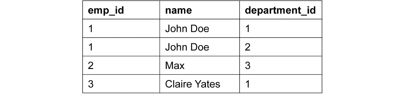
   Here, emp_id with a value of 1 has got two departments, which is not a valid form. So, to accommodate and maintain the validity, we will store the data like so:

   

   Figure 5.19: Invalid schema – table displaying the department column with multiple values

   Valid schema example

   In the following example of a valid schema, we have created a separate record for John Doe by splitting the department column values, such as IT and Pre-sales, into two different rows:

   

   Figure 5.20: Valid schema in 1st Normalization form

2. 2nd Normalization form

   This form tells us that the table should be in 1st Normalization form and that all the columns should be fully dependent on the primary key.

   Let's take an example of the performance of employees.

   Invalid schema example

   In the current example, the primary key is emp_id but the location is dependent on the department. This schema holds the information in the location column, which does not depend on the key column, emp_id, so there is a partial dependency here. Each department has a specific location, so emp_id is partially dependent on location. If we maintain department and location with employee ID in the same table, it will create redundancy of data:

   

   Figure 5.21: Invalid schema – partial dependency

   To achieve the necessary validity and remove partial dependency, we will store the data as shown in Figure 5.22 and Figure 5.23, respectively.

   Valid schema example

   The schema creates a department table to remove the partial dependency. Here, the location is dependent on department_id, which can be seen in the following table:

   

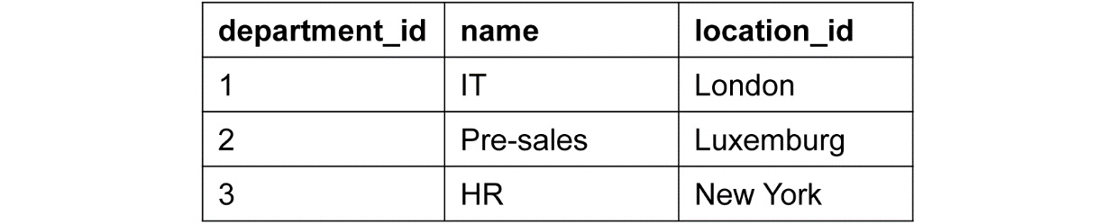
   Figure 5.22: Department table to remove the partial dependency

   So, now, we have two tables, department and employee. department_id and emp_id stand as the primary keys for the department and employee tables, respectively. With the previously mentioned approach, we removed the partial dependency by only having department_id in the employee table:

   

   Figure 5.23: Valid schema in 2nd Normalization form

3. 3rd Normalization form:

   This form says that the schema should be in 2nd Normalization form and that transitive dependencies should not exist in the single table. A transitive dependency is if A determines B (A-B) and B determines C (B-C) so that A determines C (A-C).

   Invalid schema example

   This schema shows that a transitive dependency such as emp_id determines delivery_status and that delivery_status determines performance_label, which is a transitive dependency and is not valid for the 3rd Normalization form. Let's elaborate more by explaining the components of the table. If John Doe delivers the package on time, he is meeting his set expectations. But if he delivers it before the given time, this infers that he has exceeded his expectations. The same scenarios are taking place for Max and Claire Yates as well. So, based on the delivery statuses of John, Max, and Claire, we can understand their performance labels. Since this is a transitive dependency, it is not a valid 3rd Normalization form:

   

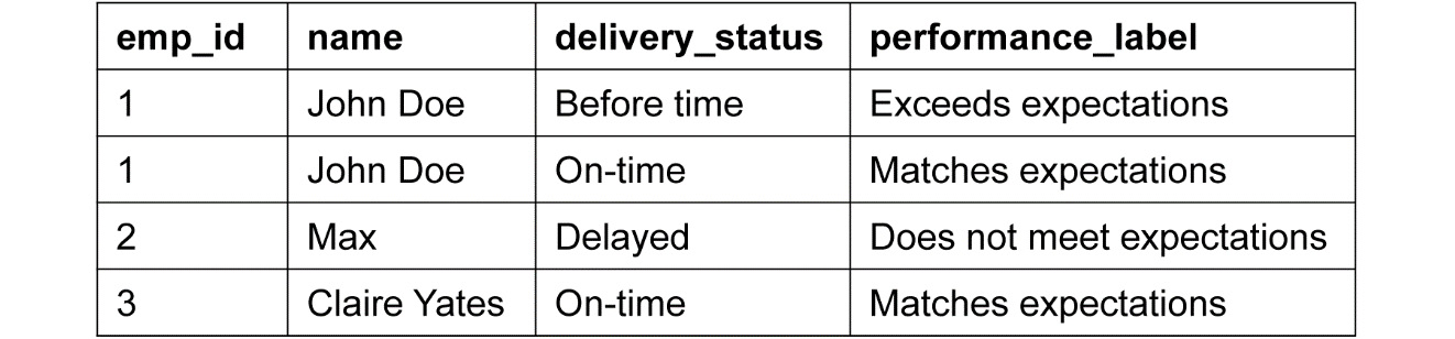
Figure 5.24: Invalid schema – transitive dependency

Valid schema example

This schema creates a delivery table to measure performance, eliminate transitive dependency, and remove duplicity, as shown in the following table:

Figure 5.25: Delivery table to remove the transitive dependency

Now, emp_id only determines delivery_status_id. delivery_status is stored in the delivery table, altogether forming a valid schema, as shown in the following table:

Figure 5.26: Valid schema in 3rd Normalization form

Dimensional Data Modeling

This technique is used while building a data warehouse. It consists of facts and dimensions. Dimensions are categories of the data and their information; for example, Time, Place, and Company. These dimensions are used to build the fact tables that contain the metrics.

There are two types of data models/schemas in dimensional data modeling:

1. Star schema

   In this, there is a fact table at the center of the star, followed by several associated dimension tables. As per its similarity with the star structure, it is referred to as a star schema. It is the simplest type of data warehouse schema and is optimized for querying large datasets. In this schema, the dimension tables do not have interrelationships, so they only interact through the Fact table:

   

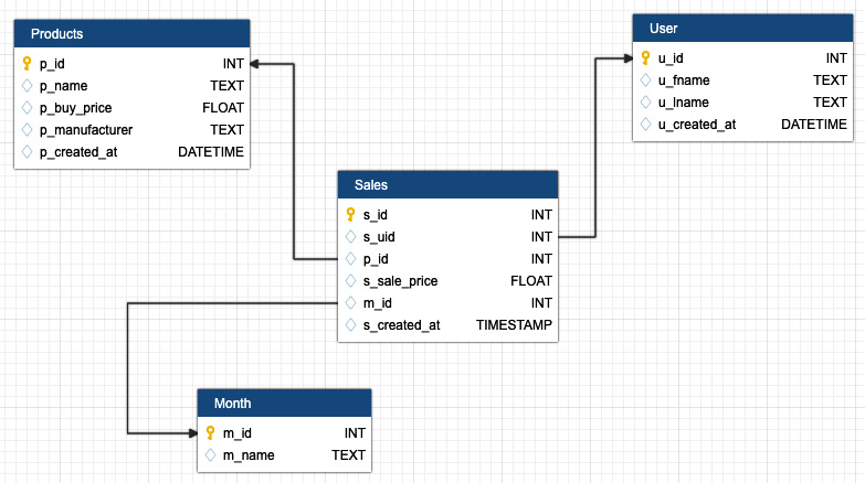
   Figure 5.27: Star schema

2. Snowflake schema

   In this schema, the dimensions can be interconnected to form the Fact table. It looks just like a snowflake, which is complex looking. This is used where complex schemas are integrated to form a bigger family:

   

Figure 5.28: Snowflake schema

These popular modeling techniques are key to successful and future-proof database design, although these tricks won't solve problems such as having a huge number of records. We will discuss this later in this chapter.

The star schema is an appropriate choice when only a single join creates a relationship between the fact table and any dimension tables, whereas the snowflake schema is an appropriate choice when there is a requirement to have many joins to fetch the data. To simplify this, if we want to design a simple database, then the star schema is appropriate, whereas the snowflake schema is an appropriate choice for designing a complex database.

Now that you know about relational database design, modeling, and its implementation, let's talk about performance tuning.

Performance Tuning and Best Practices

Companies such as Facebook use MySQL to deal with petabytes of data, but it's difficult to achieve such performance with default settings and configuration. So far, we have set up a model using SQL queries. However, it is quite understandable that by getting more products, the entries in tables of e-commerce sites such as FashionMart will also be increasing. In such a scenario, the expectation from the databases would be to perform at the same durability and speed. To ensure that, we need to tune the performance of our commands. Some of the best practices to ensure performance tuning are as follows:

• Try to avoid using SELECT *:

  Instead of selecting all the columns unless required, try to mention column names in the SELECT clause. This will lower the unnecessary overhead on the MySQL query engine.

• Limited use of the ORDER BY clause:

  ORDER BY orders the results in ascending or descending order, but this also impacts the performance of MySQL since before showing the results, they need to be sorted.

• Use LIMIT OFFSET for pagination:

  Many web applications use pagination to show records batch by batch. You can use LIMIT and OFFSET to skip and limit the records you want to show. This will improve query performance since you don't need to bring in all the records from the result.

• Sub-queries are expansive:

  Sub-queries put extra load on the query engine. Instead, use joins if possible, which are treated as part of the same query.

• Use UNION ALL instead of UNION:

  UNION combines two query results and removes duplicates, which are classed as overhead for the query engine. UNION ALL does not remove duplicates and instead leads to better performance.

• Join on numerical columns:

  Always try to perform a join on a numerical column instead of a text column as this will save a lot of time.

• Don't use too much indexing:

  A database index is a data structure that improves the speed of data retrieval operations on a database table by taking a search key as input. Indexing returns a collection of matching records efficiently. It is used to quickly locate and access the data in the database. Indexes provide good performance, but too many of them will spoil the show as every index needs to be maintained and modified for every change in the data.

These tips and practices can be used to implement production-ready MySQL databases, where you can deal with a large number of queries. We'll implement some MySQL queries in the following activity.

Activity 5.01: Managing the Inventory of an E-Commerce Website Using a MySQL Query

Imagine we have a globally successful e-commerce site for the PacktFashion store. PacktFashion is facing tough challenges to manage the products in its stock. As products are being sold out quickly, PacktFashion is unable to maintain the inventory status. One of the customers who is staying in Prague needs a quick delivery and would like to know whether their product is available in the nearby warehouse. PacktFashion is facing trouble resolving the customer's query related to product availability in stock.

This activity aims to implement a data model so that we manage the inventory of the site. We will be listing those products that are in and out of stock. Furthermore, we need to find the list of available products in the warehouse of Prague.

You need to implement the data model as shown in the following screenshot. This model will help us manage the products, sales, inventory, manufacturer, the status of the product, and the warehouse location:

Note

We have created a data model based on the snowflake schema. You can use another approach if you prefer. It should be in its 3rd Normalization form at a minimum.

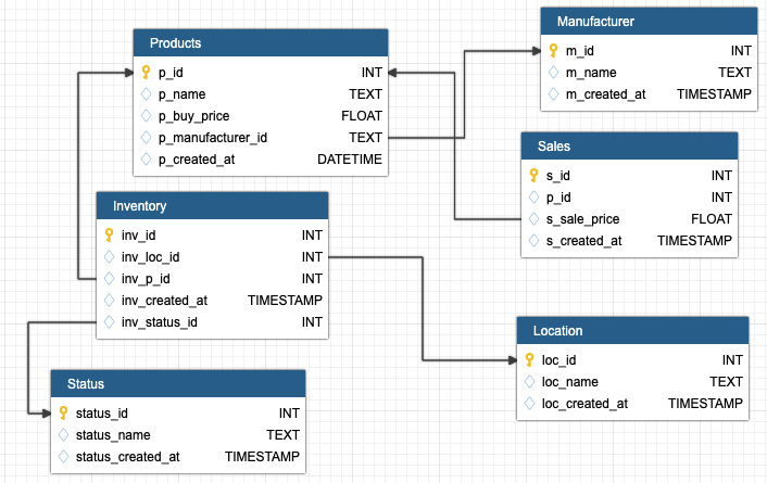
Figure 5.29: Data model using the snowflake schema

Note

The code for this activity can be found here: https://packt.live/2Wvf9xB.

Perform the following steps to complete this activity:

1. Create and use the PacktFashion database.
2. Create the necessary tables based on the data model using the PRIMARY KEY, FOREIGN KEY, and ON DELETE CASCADE queries.
3. Add at least three records for each table.

   Note

   The location table and products table must have Prague and XIMO Trek shirt as one of their records. Also, the status table should have values of IN or OUT only.

4. View the data of all the tables using the SELECT query.

   The data in the tables should be similar to the following outputs:

   

   Figure 5.30: Table data for the fashionmart data model

5. Find the total number of products in the inventory using the JOIN clause, where status_name ='IN'.

   You should get an output similar to the following:

   

   Figure 5.31: Table showing the total of in-stock products

6. Find out the total number of products that are not in the inventory using the JOIN clause, where status_name ='OUT'.

   You should get an output similar to the following:

   

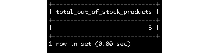
   Figure 5.32: Table showing the total of out-stock products

7. Find the status of the XIMO Trek shirt product for the Prague location.

   You should get an output similar to the following:

   

Figure 5.33: Table showing the status of the product

We have completed the SQL databases section. Now, designing and implementing relational data models and querying them should not feel like a difficult task.

We'll learn about NoSQL databases in the next section.

Note

The solution to this activity can be found on page 598.

NoSQL Databases

In the previous section, we looked at how SQL databases are used in the industry, along with some examples. However, with all the great things SQL databases can do, there is still significant room for improvement when it comes to dealing with complex and huge data with quick retrieval requirements. The times before and after NoSQL databases were created can be seen in the following diagram:

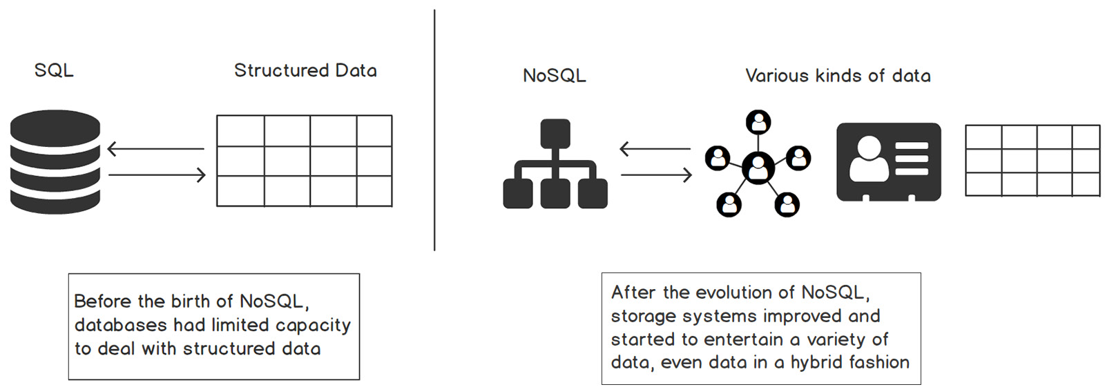
Figure 5.34: NoSQL database formats

These NoSQL databases evolved because of the fundamental limitations of SQL databases. The data in almost every sector has grown exponentially over time and the variety of usage has also expanded. Earlier, databases were limited to enterprise resource systems, research projects, telecommunications, and so on, but today, new domains have emerged with huge data in a variety of formats, such as social media and profiling millions of users, oil and gas, with billions of binary records, e-commerce, and life sciences. Because of the single server system, complex schemas, and the expense of vertical scaling, it became difficult for SQL databases to cope with high-performance requirements.

SQL databases such as RDBMS have a fixed, static, or predefined schema and these databases are not suited for hierarchical data storage, which is why these databases are best suited for complex queries. On the other hand, NoSQL databases are non-relational or distributed database systems. They have a dynamic schema. These databases are best suited for hierarchical data storage and are not very good for complex queries.

Need for NoSQL

NoSQL databases are distributed databases built and supported in various languages.

There are various kinds of NoSQL databases available. Some of the most popular include document store, columnar, key-value store, and graph databases. Let's take a look at them:

• All of these databases can handle terabytes to petabytes of data in a distributed fashion, which helps in achieving a latency of a few milliseconds, such as the data we see in Amazon, Twitter, Facebook, and Google.
• There is a developer-friendly abstraction layer built by the communities of respected databases to deal with data smoothly. A lot of companies contribute to the community to come up with the abstraction layer. For example, Facebook invented Hive to deal with Hadoop data using a SQL-like language.
• The distributed database makes it easy to scale horizontally if data grows and also makes it highly fault-tolerant.
• The majority of databases are open source, which is why they are picked by the industry.
• The decision of which database to use is taken based on the use case at hand; for example, if you want to store/analyze the logs or profile products or users, then MongoDB is the best choice since it treats each record as a document with a flexible schema.

We will discuss document store and columnar databases and provide examples in the following sections. Before we dive into NoSQL in more detail, let's have a careful look at one of the most important big data theorems: CAP theorem. This theorem is used to set the agenda for the data storage system.

Consistency Availability Partitioning (CAP) Theorem

This theorem is the de facto standard for deciding on the most appropriate NoSQL data storage:

• Consistency: This is the same concept we studied in ACID properties; it is about maintaining the same state of the data at any given point in time.
• Availability: This concept is about the system or, specifically, speaking data being available, even during node/cluster failures so that successful reads and writes can take place.
• Partitioning: According to this concept, the data is partitioned across the network as a secondary source in case of network congestion or node failures:

Figure 5.35: CAP theorem

As shown in the preceding diagram, the databases that give good consistency and fair availability are relational databases/SQL databases. One of the databases that can guarantee partitioning and availability is Cassandra. Some of the databases that have a good mixture of consistency and partitioning include HBase, MongoDB, and Redis.

So, with this theorem, the following is clear:

1. If you partition the data, then it's difficult to sync the state of data (that is, Consistency), but the data is available all the time. This is known as AP (Availability and Partitioning).
2. If you sync the data between its copies (joins), then there is a chance of a single point failure occurring, but the state of data can be maintained easily. This is known as CP (Consistency and Partitioning).

So, ideally, only two designs (we call this an agenda) can be chosen (either CP or AP) while considering data storage. Let's start with CP and learn how it's implemented through the MongoDB database.

MongoDB

MongoDB is a document-oriented database and is a generalized form of the NoSQL database. This database is popular among the community, especially for use cases such as logging, user profiling, search engines, geolocation data, and configuration storage.

It solves the scalability limitation of relational databases with its distributed architecture. So, it is considered an alternative to SQL databases. The installation and implementation of MongoDB is quite easy. For instance, Coinbase (digital currency exchange) uses MongoDB to build faster applications, diversify data type handling, and for efficient application management purposes. Let's now discuss the advantages and disadvantages of MongoDB.

Advantages of MongoDB

• Since MongoDB stores, the data in consecutive memory locations, querying for one of the fields of the whole document can be retrieved from memory quite easily. Hence, MongoDB does not need to look through the whole disc.
• It supports complex data types, such as Map and List.
• It is a distributed database, which means we can set up a cluster of MongoDB with the Master-Slave paradigm. This cluster partition replicates the data to provide low latency and high availability.
• It's a schema-less database, which means that the collection adopts the schema based on the data that's inserted. So, when you are not sure about the schema, MongoDB is the right choice for such a scenario.
• It comes with a powerful query engine for NoSQL queries using JavaScript.

Disadvantages of MongoDB

• MongoDB does not support joins to ensure high availability.
• Relational data modeling approaches are not useful with MongoDB.
• Partitioning and denormalization lead to data duplication and data inconsistency.
• No default transaction support, so users need to handle these issues by themselves.

Query Language

The query language that's used for MongoDB is JavaScript. The MongoDB team has provided a variety of functions to deal with collections and data.

Terminology

As we discussed previously, you must be aware of SQL terminology. We will try to align the terminology of MongoDB with the former to aid our understanding:

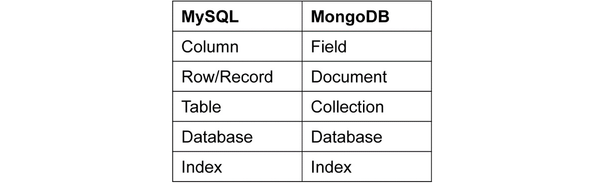
Figure 5.36: Comparison of MySQL and MongoDB terminology

Now, let's talk about the functions of the newly created sales MongoDB collection:

• Use

  Databases are selected through the use command:

  use fashionmart

  show dbs

  If you create the collection here, only the database is created.

• Create Collection

  db.createCollection("Sales")

  This function creates the collection with the sales name in the fashionmart database.

• Insert

  You can create a JavaScript object and insert it into the collection:

  db.Sales.insert(<JavaScript object or JSON object)

  Multiple records can be combined in this object:

  db.Sales.insert(

   [

   {

   "ShirtID":"1",

   "ShirtColor":"2",

   "ShirtSize":"XL",

   "ShirtDetails": [

       {

          "styleID": "4",

          "designerID": "6",

       }],

   },

   {

   "ShirtID":"2",

   "ShirtColor":"Red",

   "ShirtSize":"XXL",

   "ShirtDetails": [

       {

          "styleID": "5",

          "designerID": "6",

       }],

   }

   ]

   );

• Find

  This function can be used to find the records from the collection:

  db.Sales.find({ShirtID:"2"}).pretty()

  It should give us the following output:

  

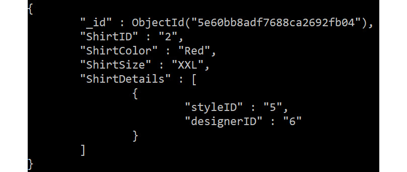
Figure 5.37: Finding a query on the records of a collection

Here, we are querying the sales collection with the ShirtID criteria (the where clause in MySQL) as 2. The pretty function at the end displays the output JSON in a structured way. Here, the pretty() method is used mainly to display the result in an easier-to-read format.

Let's take another example of searching for an element value in an array and implement it using the Find query and then, alternatively, with the $elemMatch operator:

db.Sales.find({"ShirtDetails.styleID":"4"}).pretty()

It should give us the following output:

Figure 5.38: Finding a query on the records of a collection

Alternately, you can use the $elemMatch operator, as follows:

db.Sales.find({ShirtDetails: {$elemMatch :{ styleID:"4"}}}).pretty()

It should give us the following output:

Figure 5.39: The $elemMatch operator as an alternative to the Find query

Both commands will retrieve the whole matching document.

• Aggregate

  In MongoDB, aggregation pipelines are a breakthrough. Using these, you can chain various operations, such as grouping, aggregation, and exploding the embedded document. Here, operations such as "exploding the embedded document" imply the deconstruction of an array field from the input documents to the output document for each element.

  It is not a standard practice to use hardcoded values such as column name, alias name, and even the column that we want to perform the count on. To solve this, we can create JavaScript functions that are dynamic and return an object depending on the arguments so that we don't have to rely on the hardcoded values.

  Let's understand this through an example:

  db.Sales.aggregate([{$unwind: "$ShirtID"}]).pretty();

  It should give us the following output:

  

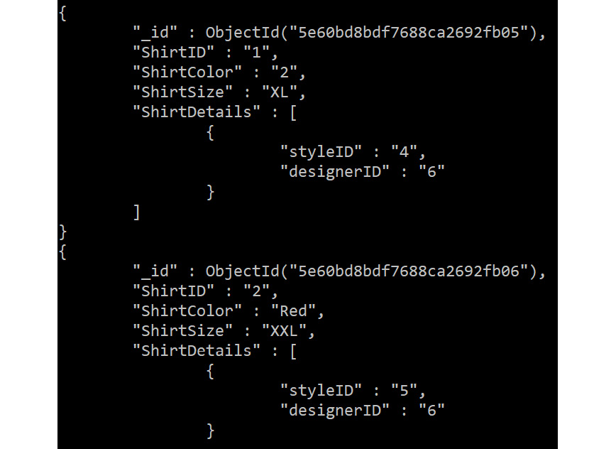
Figure 5.40: Aggregate query on the Sales collection

• Pipeline concept

  Here, we are using a JavaScript function that returns the aggregate pipeline object:

  function sales_designer(match_field, match_value) {

  var matchObject = {};

  var eq_object = {};

  eq_object["$eq"] = match_value

  matchObject[match_field] = eq_object

  return [

        {

          "$unwind":"$ShirtDetails"

        },

        {

          "$match": matchObject

        },

        {

          "$project": {

             "StyleID":"$ShirtDetails.styleID"        

           }

        }

       ]

   };

  The JavaScript function executes in the following sequence:

• $unwind explodes/deconstructs the ShirtDetails array to each individual element and then uses them.
• $match filters the result over match_field equal to match_value, which is given as a parameter in the function.
• $project is just like the SELECT clause in relational databases, returning just styleID from ShirtDetails.

  Note

  Other criteria can also be parameterized and used as input in the pipeline function.

  In this example, the $unwind operator in MongoDB has been used to deconstruct an array field from the input documents to the output document for each element:

  db.Sales.aggregate(sales_designer("ShirtDetails.designerID","6")).pretty()

  It should give us the following output:

  { "id" : ObjectID("5e60bd8bdf7688ca2692fb05"), "StyleID" : "4" }

  { "id" : ObjectID("5e60bd8bdf7688ca2692fb06"), "StyleID" : "5" }

  This command runs this pipeline and executes the commands in a sequence of declaration.

To understand MongoDB better, we will look at a simple example. For ease of understanding, we will be using the FashionMart example.

Imagine that you want to build a report for each product and that there are thousands of products in the inventory. Each product has millions of sales. If we need to build the solution using a relational database, then it will be a combination of the product's dimension and its sales, and the query will include a join between these two. This will result in extensively scanning and mapping each product to its sales data. In the case of a billion sales records for over a hundred thousand products, this join would be complex, which makes it an expensive solution. Another major drawback would be the query being performed on a single database server.

Now, let's think about this problem using MongoDB. As we know, joins are not encouraged, so the data will probably be in a denormalized manner. So, if we want reports for each product, the sales entity will be embedded inside the product entity. This way, we avoid joins and put data in a single collection. Also, using the aggregations in MongoDB, we can get interesting analytics out of the data.

Let's create a data model for this example. We will call the collection Product.

This collection will hold the product and sales information inside the same collection. It should look as follows:

{

"_id": "5498da1bf83a61f58ef6c6d5",

"p_name": "Z-1 Running shoe",

"p_manufacturer": "Z-1",

"p_buy_price": 34,

"p_created_at": Date(),

  "sales": [

    {

"s_sale_price": 40,

      "s_profit": 6,

      "p_created_at": Date(),

    },

    {

      "s_sale_price": 41,

      "s_profit": 7,

      "p_created_at": Date()

    }

  ]

}

In the data model, the example document is shown with an autogenerated mongo ID. Then, the sales object is added to the Sales array field. If you query for a product of Z-1 manufacturer, then without joining the collection, all the necessary information will be fetched.

We will implement this example in the next exercise using the MongoDB database.

Exercise 5.02: Managing the Inventory of an E-Commerce Website Using a MongoDB Query

In this exercise, we will implement the data model for FashionMart in MongoDB. Then, we'll display the report of a specific product, along with its sales data. Then, we will find the total products in the inventory and the bestselling product whose profit is greater than 6.

Before proceeding with this exercise, we need to set up a MongoDB database. Please follow the instructions on the Preface to install it.

Perform the following steps to complete this exercise:

1. Open the MongoDB shell:

   $mongo

   Notec

   For additional help on starting the MongoDB shell, refer to the following link: https://docs.mongodb.com/manual/mongo/#start-the-mongo-shell-and-connect-to-mongodb. For a quick reference of all the important MongoDB shell commands, visit: https://docs.mongodb.com/manual/reference/mongo-shell/.

2. Use the show query to see the list of existing databases:

   show dbs

   You should get the following output:

   admin 0.000GB

   config 0.000GB

   demo 0.000GB

   local 0.000GB

3. Create a database called fashionmart through the use query:

   use fashionmart

   You should get the following output:

   switched to db fashionmart

   Now, you can directly start using the database without creating it. It will be created when you create a collection in it.

4. Create a products collection, as shown in the following query:

   db.createCollection("products");

   You should get the following output:

   {

           "ok" : 1,

           "$clusterTime" : {

                    "clusterTime" : Timestamp(1593812618, 7),

                    "signature" : {

                           "hash" : BinData(0,"XLov2h+xWNKbYrcWIqsCOROMuKY="),

                             "keyId" : NumberLong("6808867179686002691")

                    }

            },

           "operationTime" : Timestamp(1593812618, 7)

   }

   In MongoDB, we do not have a structure for the collection, so we will start with data insertion in the products collection.

5. Insert the necessary data into the products collection. For the record, we will need today's date:

   todayDate=new Date()

   You should get the following output:

   ISODate("2019-12-21T16:05:48.765Z")

   We can also create a variable for time efficiency. Since the query language to access MongoDB is JavaScript, the way we access the interface is a mix of procedural and declarative.

6. Now, we'll create the product's JavaScript object so that it can be inserted into a collection:

   products={

   "p_name": "Z-1 Running shoe",

   "p_manufacturer": "Z-1",

   "p_buy_price": 34,

   "p_created_at": todayDate,

   "sales": [

     {

       "s_sale_price": 40,

       "s_profit": 6,

       "p_created_at": todayDate,

     },

     {

       "s_sale_price": 41,

       "s_profit": 7,

       "p_created_at": todayDate

      }

     ]

   }

   You should get the following output:

   

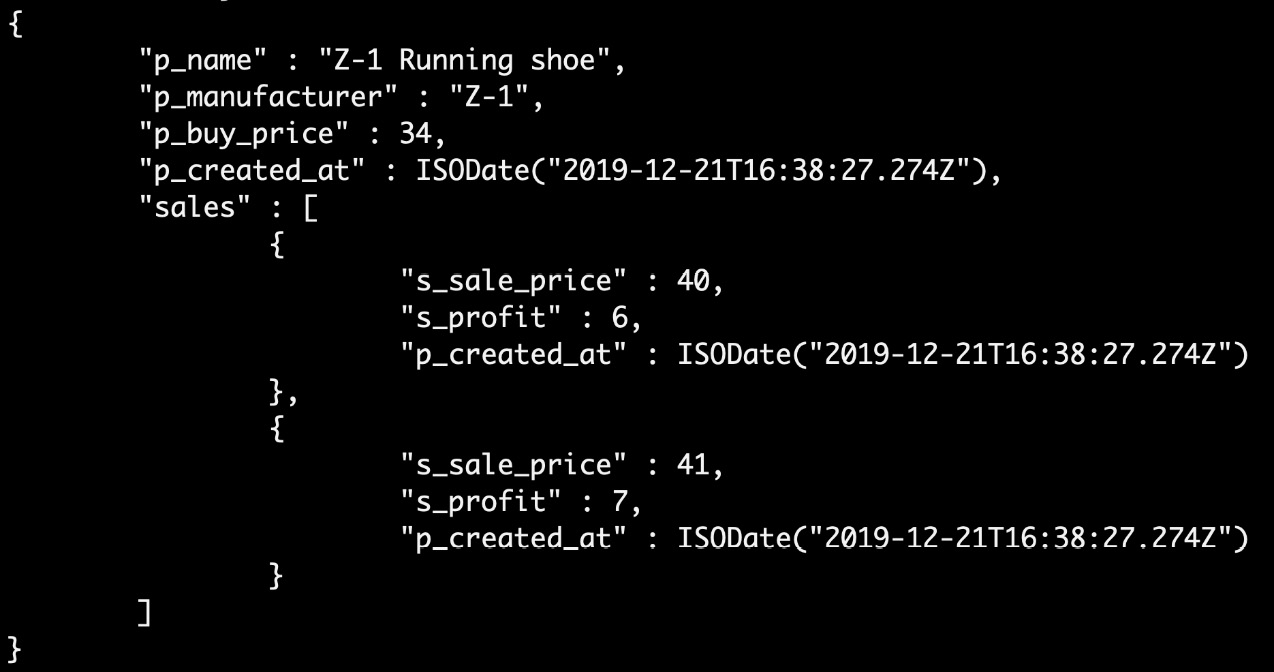
   Figure 5.41: Result

7. Lastly, insert the products object as a document in the collection:

   db.products.insert(products);

   You should get the following output:

   WriteResult({ "nInserted" : 1 })

8. Create a JavaScript script object called total_sales_for_product for "Z-1 Running shoe" to find the total units sold, as shown in the following query:

   total_sales_for_product_pipeline=[

     {

       "$match": {

         "p_name": "Z-1 Running shoe"

       }

     },

     {

       "$project": {

         "product":"$p_name",

         "total_sales": {

           "$size": "$sales"

         }

       }

     }

   ];

   With this, we have created a JavaScript array object that will hold the total_sales pipeline operations.

9. Generate a report for using the JavaScript array object with the aggregate function, as shown in the following query:

   db.products.aggregate(total_sales_for_product_pipeline).pretty()

   You should get the following output:

   {

           "_id" : ObjectId("5dfe4c0b211649ccef9a7426"),

           "product" : "Z-1 Running shoe",

           "total_sales" : 2

   }

   Here, we have filtered the records for shoe and then performed a count over the sales object field. We used the aggregate pipelining function to perform the functions. This way, various pipelines can be built as JavaScript objects and then executed to get the results.

10. Create a function called total_product_sales to parameterize the pipeline object's creation, as shown in the following query:

    function total_product_sales(match_product,

    projection_field,

    count_field) {

    var matchObject = {};

    var countObject = {};

    matchObject[projection_field] = match_product

    countObject["$size"] = "$"+count_field;

    return [

      {

        "$match": matchObject

      },

      {

        "$project": {

          "product":"$"+projection_field,

    "total_sales": countObject

      }

     }

    ]

    };

    Here, we have created a total_product_sales function that will return the desired pipeline object. You can modify this function to suit your requirements. Now, it is time to call this function inside the aggregate function.

11. Generate the report using the total_product_sales and aggregate function, as shown in the following query:

    db.products.aggregate(total_product_sales("Z-1 Running shoe", "p_name","sales")).pretty();

    You should get the following output:

    {

            "_id" : ObjectId("5dfe4c0b211649ccef9a7426"),

            "product" : "Z-1 Running shoe",

            "total_sales" : 2

    }

12. Find the total number of products in the inventory using the count function, as shown in the following query:

    db.products.count();

    You should get the following output:

    1

13. Create the gt_product_sales() function to find the products with a profit greater than 6, as shown in the following query:

    function gt_product_sales(gt_value, compare_field) {

          var gt_object = {};

          var match_object = {};

          gt_object["$gt"] = gt_value

          match_object[compare_field] = gt_object

      return [

          {

            "$unwind":"$sales"

          },

          {

            "$match": match_object

          },

          {

            "$project": {

               "product":"$p_name",

               "sales":"$sales"

             }

          }

         ]

     };

    Here, we created a JavaScript function called gt_product_sales(). This function will take gt_value and compare_field and return the JavaScript object that acts as input to the MongoDB aggregate function. Also, we used the $unwind operator to flatten the document and create one document for each element in the sales array field.

14. Find the product with a profit greater than 6 using the aggregate function, as shown in the following query:

    db.products.aggregate(gt_product_sales(6, "sales.s_profit"));

    You should get the following output:

Figure 5.42: Result of aggregate with the unwind operator

This command executes the aggregate function to get the products that have a profit greater than the given gt_value. In our case, we have passed a value of 6.

Note

To access the source code for this specific section, please refer to https://packt.live/3epAaQ0.

With that, you have addressed a problem statement in MongoDB. Now, you can start thinking of various ways to perform similar operations and try to implement that on your local instance. By implementing this exercise, we have understood the importance of MongoDB to overcome complexities while dealing with large databases. Unlike SQL, since it's a schema-less NoSQL database, there are flexibilities while storing JSON documents. So far, we've learned how MongoDB reduces the complexity of deployment by speeding up application development.

Now, let's move on to data modeling.

Data Modeling

In this section, we will discuss how to model the data for MongoDB. NoSQL data modeling is a new paradigm and MongoDB, being a document store database, saves data in BSON (Binary JSON) format. So, to make the most of MongoDB, the modeler has to think in JSON.

Let's go over the techniques of data modeling in MongoDB.

Lack of Joins

The reason why a record is called a document is that MongoDB is expected to find all the required information in one place. Imagine a real-world scenario where you are reading an important document. It's obvious that you expect to find all the information in the same document. It would be annoying if you could only read pieces of information through various documents.

To make reading over all the information as low latency as possible, MongoDB does not encourage joins in the collections. Here, we are talking about data duplication, which is a violation of normalization rules, but it is the key to quick reads from storage discs.

Let's take an example from the FashionMart use case. We created two tables, Products, and Sales. Right now, you can get sales data for a product by joining these two tables, but what if there are thousands of products and billions of sales records? Especially if you think in terms of distributed computing, the Sales table data is partitioned and stored in various machines in the cluster, so when you join the records of Products and Sales, then there will be a large amount of data transfer, as shown in the following diagram:

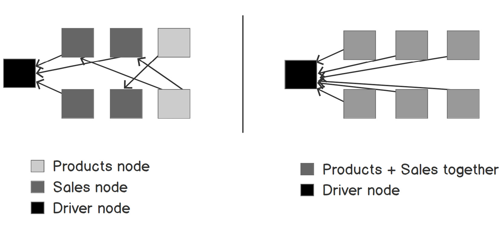
Figure 5.43: Two scenarios performed with and without joins in collections

On the left-hand side, let's assume that the Products and Sales data is stored in separate collections, that is, separate nodes. As you can see, there is a lot of data exchange over the network because of the joins. However, on the right-hand side, the Products and Sales data is together, so there are no joins. This means that less data exchange happens over the network.

The resulting data model will be of the embedded type, where the Sales data will be embedded in the Products collection, as shown in the following query:

{

    "_id":ObjectId("5dfe4c0b211649ccef9a7426"),

    "p_name":"Z-1 Running shoe",

    "p_manufacturer":"Z-1",

    "p_buy_price":34,

    "p_created_at":ISODate("2019-12-21T16:38:27.274Z"),

    "sales":[

        {

            "s_sale_price":40,

            "s_profit":6,

            "p_created_at":ISODate("2019-12-21T16:38:27.274Z")

        },

        {

            "s_sale_price": 41,

            "s_profit":7,

            "p_created_at":ISODate("2019-12-21T16:38:27.274Z")

        }

    ]

}

Joins

MongoDB is designed not to have joins, which is why there are two workarounds for this application: side joins and out-of-the-box joins. These are new concepts where you maintain SQL-like relationships between MongoDB collections. Joins have to be performed by the application layer. Let's have a look at one such example:

products

{

    "_id":ObjectId("5dfe4c0b211649ccef9a7426"),

    "p_name":"Z-1 Running shoe",

    "p_manufacturer":"Z-1",

    "p_buy_price":34,

    "p_created_at":ISODate("2019-12-21T16:38:27.274Z"),

}

Sales

{

    "_id":ObjectId("4dfe4c0b475649ccef9a7426"),

    "s_sale_price":40,

    "s_profit":6,

    "s_created_at":ISODate("2019-12-21T16:38:27.274Z")

    "p_id":ObjectId("5dfe4c0b211649ccef9a7426")

},

{

    "_id":ObjectId("2dfe4c0b475649jfkf9a7426"),

    "s_sale_price": 41,

    "s_profit":7,

    "s_created_at":ISODate("2019-12-21T16:38:27.274Z")

    "p_id":ObjectId("5dfe4c0b211649ccef9a7426")

}

It should give us the following output:

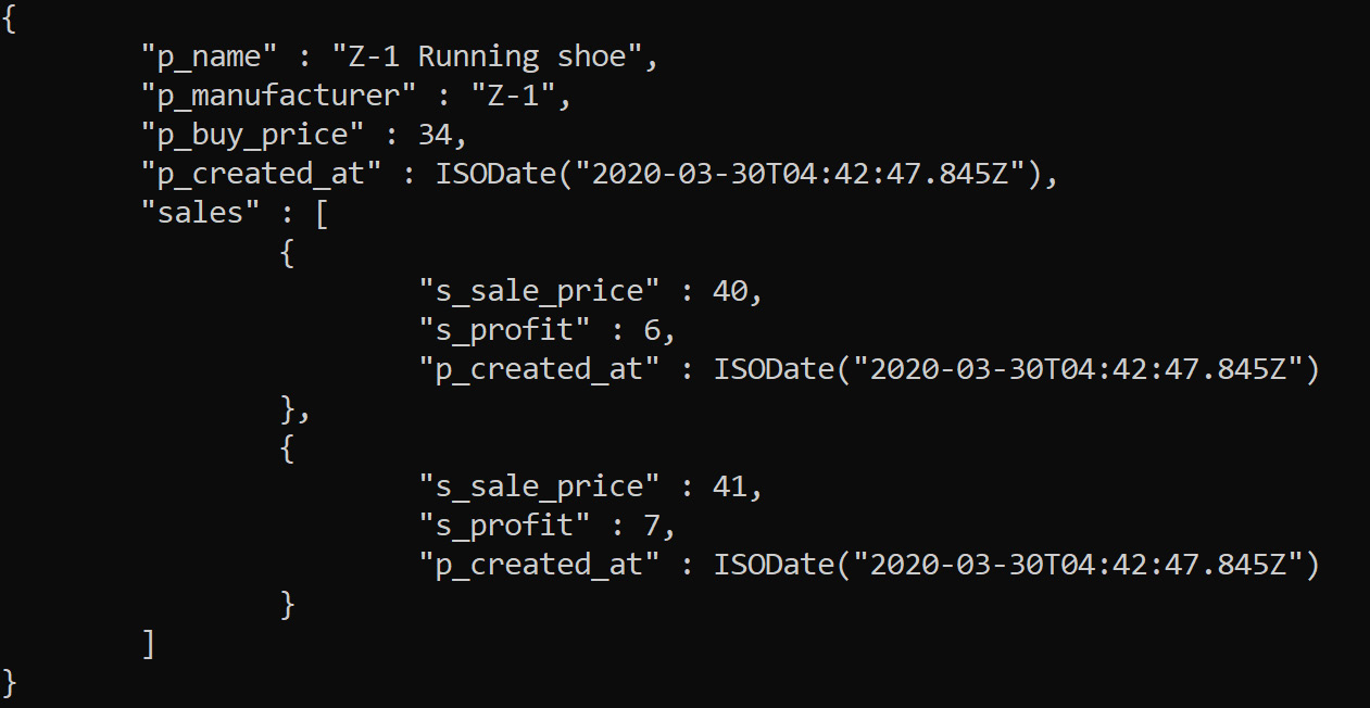
Figure 5.44: Joins in MongoDB

The procedure to join these two collections is to take the product's ID and query the sales collection against the matching p_id field. In this case, we can create an index for the p_id column so that it can be retrieved and matching can be made simpler. This can be made possible at the application layer in a programming language by taking an ID from a collection and searching the records of the target collection based on the ID. You can also use the $lookup operator with the aggregate pipeline to join the two collections.

With that, we have covered the various techniques of data modeling in MongoDB. There's lots of domain-specific variety that can be used for the respective domains.

Performance Tuning and Best Practices

To make the database production-ready, there are some tricks to consider:

• Use the aggregation pipeline as much as possible since it's an in-built function that utilizes MongoDB functionality properly.
• Use less embedding by flattening the records if possible. This results in a major drop in latency.
• Use indexes wisely; indexing on textual columns occupies lots of storage.
• Use bulk operation where possible, such as bulk insertion and reading through code, to reduce network traffic.
• Whenever possible, perform lookups following the limit operation in the aggregation pipeline.
• Embedding hampers the insertion of records. For write-heavy applications, consider using the join method referenced to improve write latency.
• MongoDB is a very good fit for production-scale applications with huge data (that is, petabytes).

Using these techniques, you can build a high-performing MongoDB instance. How you use your resources is more important than what resources you use.

Activity 5.02: Data Model to Capture User Information

Let's take the example of a globally successful e-commerce site for the PacktFashion store. PacktFashion is facing tough challenges with managing the user logs on their site. They want to store users who are either visitors or buyers on their site so that they can send them sale offers in the future.

This activity aims to add product information and store information about users and their logs on our website. Furthermore, we will generate a report to show the user, along with the products they view, and the action (bought or not bought) that was performed by them.

You need to implement the data model shown in the following screenshot. The user_logs collection will store the events performed by the users, that is, whether they bought or returned a product. The many-to-many relationships between products and users are shown in this collection:

Figure 5.45: Data model for UserLogs

Note

The code for this activity can be found here: https://packt.live/2ZlIZGy.

Perform the following steps to complete this activity:

1. Create and use the PacktFashion database.
2. Create a Products collection and add data to it.

   The data in the collection should be similar to the following output:

   

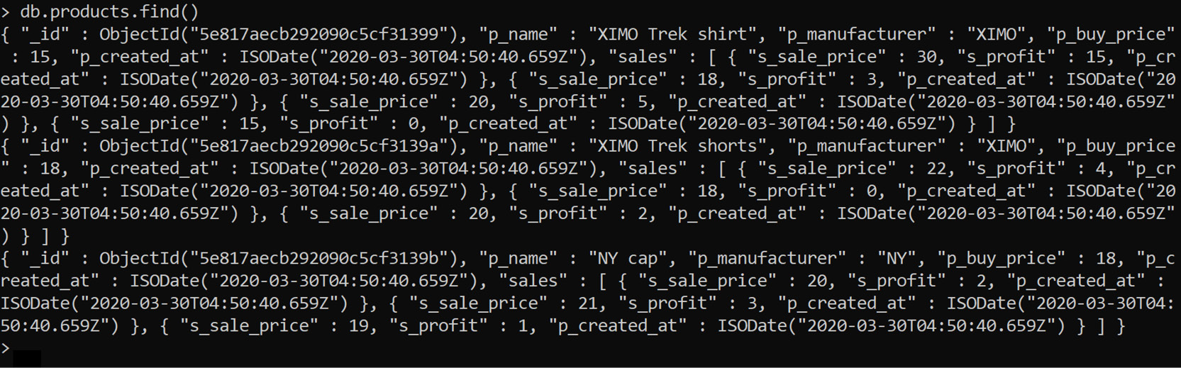
   Figure 5.46: Products collection

3. Insert an object for Products.
4. Create users and user_logs collections based on the data model.

   The data in the collections should be similar to the following outputs:

   

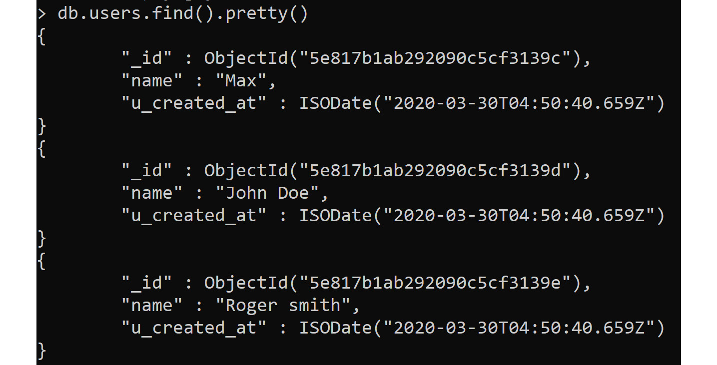
   Figure 5.47: The users collection

   

   Figure 5.48: The user_logs collection

5. Insert objects for the user and user_logs collections.
6. Join the user and user_logs collections using an aggregate function.
7. Generate the report of user logs using $lookup.

   You should get the following output:

   

Figure 5.49: Using $lookup to join the collections

With this activity, we've completed the MongoDB section. We have successfully learned about MongoDB's design, its implementation, and how it differs from relational databases. Now, let's move on to the next NoSQL database, Cassandra.

Note

The solution to this activity can be found on page 606.

Cassandra

The topic of NoSQL isn't complete without discussing columnar storage. In Cassandra, the data is stored and read in columns instead of rows. Each column is stored separately with the same row offset related to the table. We will study offset in the Data Modeling subsection:

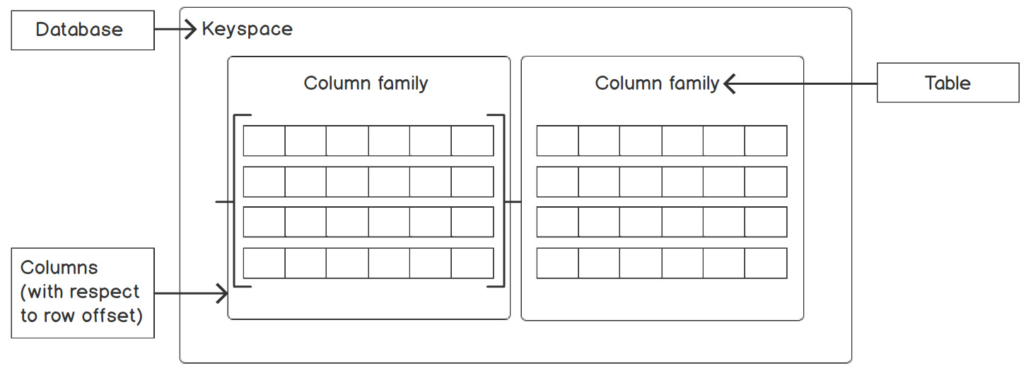
Figure 5.50: Keyspace and column family internal structure

Cassandra is a mixture of structured data, consistency, high scalability, and no single point of failure, and also has a powerful column family design. This particular database was developed by Facebook in 2008 and is horizontally scalable. Imagine you run a multinational company. You have thousands of employees, but you want the information of all the employees at the London location. In such a scenario, a traditional relational database will scan each row, parse it, and compare the u_location column value against the query. This is extremely time-consuming.

On the other hand, the columnar store only requires columns to operate. It not only saves resources but reduces the query processing time as well.

Advantages of Cassandra

• Saves metadata for each column due to its columnar format design.
• Fetches the required columns into memory, avoiding full table scans.
• Efficient for micro writes and analysis queries.
• Highly scalable.
• No single point of failure (SPOF) due to a replication functionality of two or more.
• Open-source database.
• Capable of grouping columns into a family. This means that you can retrieve specific groups simultaneously rather than individual columns.
• Uses languages with SQL-like semantics to deal with data. This is known as the Cassandra Query Language (CQL). It was developed to make learning easy since the majority of people only know SQL.

Disadvantages of Cassandra

• Source replication means bad data is also replicated across clusters, which needs to be corrected.
• Data duplication due to denormalization.
• No validation, such as constraint checks and unique values.
• Steep learning curve to making it production-ready.

Dealing with Denormalizations in Cassandra

Let's look at an example where denormalized user data is stored in a user table and then converted into columnar format, as shown in the following diagram:

Figure 5.51: Columnar format representation

Now, each column is stored separately with metadata and offset the same as a row. The table user is converted into a columnar format where each column is separate, where, if queried with u_fname, then only u_id and u_fname will be brought into memory.

Query Language

The query language that's used for Cassandra is CQL. Let's go over the terminology associated with it.

Terminology

Just like how we understood the terminology of MongoDB, we will do the same to find out more about the key concepts of Cassandra. Before we dive into an example, we should know the basic terminology and concepts:

Figure 5.52: Comparison of MySQL and Cassandra terminology

The Cassandra terminology is similar to that of the relational database:

Figure 5.53: Cassandra terminology

• Keyspace

  This is the collection of tables and column families as it stores all of its columns separately. There is one keyspace per node in a cluster.

  Keyspace has two attributes, Replication, and Durable Writes, which gives us the freedom to configure a particular keyspace. Let's understand replication first.

  Replication has two options, as shown in the following table:

  

Figure 5.54: Replication properties table

Durable write

If this is set to TRUE, then Cassandra maintains an update log for every data modification so that if the system crashes, we have the logs of the data to recover. The default value is TRUE; it should be kept as the default if possible. Just to show an example, we have added some syntax to change it to false.

Let's create a keyspace called fashionmart to understand replication and durable write better, as shown in the following code:

CREATE KEYSPACE fashionmart

WITH replication = {'class':'SimpleStrategy',

                    'replication_factor': 3}

                    AND DURABLE_WRITES = false;

DESC keyspaces;

USE fashionmart;

Here, 'SimpleStrategy' stands for "Strategy name" and describes a simple replication factor for the cluster. The replication factor value is 3.

• COLUMNFAMILY

  This is like a table in that it is a collection of columns. You can create a ColumnFamily like so:

  CREATE COLUMNFAMILY user(

  u_id int PRIMARY KEY,

  u_fname text,

  u_lname text,

  u_age int,

  u_location text,

  u_created_at timestamp,

  u_last_visited timestamp);

  It should give us the following output:

  

Figure 5.55: Stdout to the CREATE KEYSPACE command

Just like a relational database, you will have to specify column names and data types.

• DATA RETRIEVAL

  You can use the SELECT clause to retrieve records from COLUMNFAMILY. The Cassandra query engine locates the column with a byte offset and brings only the specified column into memory. This saves a lot of overhead while filtering the records:

  SELECT u_fname, u_lname, u_age FROM user;

  The SELECT query retrieves u_fname, u_lname, and u_age from the user COLUMNFAMILY.

Just like relational databases, you can also use aggregate functions, such as SUM, AVG, MIN, and MAX. This way, you can deal with data inside Cassandra using CQL.

Let's understand Cassandra in more detail using an example.

We have been discussing the FashionMart use case in this chapter and it has evolved from being a simple products and sales model to a SQL normalized model that has a searchable NoSQL design. Now, we will discuss the user side of it. We'll assume that there will be millions of users accessing this website, so we need to store their information to understand our audience better.

In this example, we need to store the user table in such a way that it can store the data of millions of users and give us access to the data with very low latency and high availability. Normally, with a relational database, this kind of table requires an index, but when querying an unindexed column that has this many records, it can take a lot of time to retrieve the data.

Instead of this, we will utilize the Cassandra columnar storage format, where each table will be stored separately in a column family. Let's implement this in the next exercise.

Exercise 5.03: Managing Visitors of an E-Commerce Site Using Cassandra

Let's take the previous problem statement where we need to store user information in a Cassandra column family called user. This exercise aims to store the number of visits that users have made to the site and perform queries on it. We will find the maximum and the minimum number of visits, along with the average age of the user.

Before proceeding with this exercise, we need to set up the Cassandra database. Please follow the instructions on the Preface to install it.

Perform the following steps to complete this exercise:

1. Launch the Cassandra CLI based on your OS, as shown here:

   Windows:

   Open Cassandra CLI application

   Linux:

   root@ubuntu: -$ cqlsh

   macOS:

   MyMac:~ root$ cqlsh

   You should get the following output:

   cqlsh>

   Note

   If you are having issues starting Cassandra CLI, you may try starting it with the cassandra -f command. For installation instructions for Cassandra on Windows 10, you can refer this link: https://medium.com/@sushantgautam_930/simple-way-to-install-cassandra-in-windows-10-6497e93989e6. For installation instructions on Linux, you can visit https://cassandra.apache.org/doc/latest/getting_started/installing.html.

2. Create and select the fashionmart keyspace, as shown in the following query:

   CREATE KEYSPACE fashionmart

   WITH replication = {'class':'SimpleStrategy',

                       'replication_factor' : 3};

   use fashionmart;

3. Create a COLUMNFAMILY called user, as shown in the following query:

   CREATE COLUMNFAMILY user(

   u_id int PRIMARY KEY,

   u_fname text,

   u_lname text,

   u_age int,

   u_location text,

   u_created_at timestamp,

   u_last_visited timestamp);

4. Check whether the user column family was created in the fashionmart keyspace using the following query:

   DESC tables;

   You should get the following output:

   user

5. Check the user column family using the SELECT clause:

   SELECT * FROM user;

   You should get the following output:

   

   Figure 5.56: User column family results

   Column families in Cassandra are any group of columns, be they a table or an actual family. Now, let's add data to it.

6. Insert the sample data into the user column family, as shown in the following query:

   INSERT INTO user(u_id, u_fname, u_lname, u_age,

                    u_location, u_created_at,

                    u_last_visited)

   VALUES(1,'Derek', 'Gates', 18, 'San Francisco',

          toTimestamp(now()), '2019-10-30 12:05:00+0000');

7. Now, insert the records in batches, as shown in the following query:

   BEGIN BATCH

     INSERT INTO user(u_id, u_fname, u_lname, u_age,

                      u_location, u_created_at,

                      u_last_visited)

     VALUES(2, 'Max', 'Frost', 15, 'London', toTimestamp(now()),

          toTimestamp(now()));

     INSERT INTO user(u_id, u_fname, u_lname, u_age,

                      u_location, u_created_at, u_last_visited)

     VALUES(3,'Isabela', 'McGuire', 29, 'Seattle',

          toTimestamp(now()), '2019-11-07 07:30+0000');

     INSERT INTO user(u_id, u_fname, u_lname, u_age,

                      u_location, u_created_at,

                      u_last_visited)

     VALUES(4,'Roger', 'Moore', 68, 'Amsterdam',

          toTimestamp(now()), '2019-12-02 14:50+0000');

   APPLY BATCH;

8. View the user column family's data using the SELECT query:

   SELECT * FROM user;

   You should get the following output:

   

   Figure 5.57: User column family data

9. Add the u_visits column to the user column family, as shown in the following query:

   ALTER COLUMNFAMILY user ADD u_visits int;

   By default, it will assign a null value to each record. Let's add the number of visits for each record with batch update statements.

10. Add some data to the u_visits column, as shown in the following query:

    BEGIN BATCH

      UPDATE user

      SET u_visits=1

      WHERE u_id=1;

      UPDATE user

      SET u_visits=21

      WHERE u_id=2;

      UPDATE user

      SET u_visits=14

      WHERE u_id=3;

      UPDATE user

      SET u_visits=18

      WHERE u_id=4;

    APPLY BATCH;

11. Confirm the data insertion of u_visits by viewing the user column family's data using the SELECT query:

    SELECT * FROM user;

    You should get the following output:

    

    Figure 5.58: User column family following the update operation

12. Find the maximum visits using aggregate functions, as shown in the following query:

    SELECT MAX(u_visits) AS max_visits FROM user;

    You should get the following output:

    

    Figure 5.59: Showing max visits

    The MAX function will find the highest value in the u_visits column and show it within the max_visits header.

13. Find the minimum visits using aggregate functions, as shown in the following query:

    SELECT MIN(u_visits) AS min_visits FROM user;

    You should get the following output:

    

    Figure 5.60: Showing min visits

    The MIN function will find the lowest value in the u_visits column and show it within the min_visits header.

14. Calculate the total number of visits, as shown in the following query:

    SELECT SUM(u_visits) as total_visits FROM user;

    You should get the following output:

    

    Figure 5.61: Showing total visits

    Here, we have used the SUM aggregation function to get the result of total visits, that is, 54 in this query.

15. Calculate the average age group of the visitors, as shown in the following query:

    SELECT AVG(u_age) as average_age FROM user;

    You should get the following output:

    

Figure 5.62: Showing average age

Here, we have used the AVG aggregation function to calculate the average age on the u_age column. We got an average age of 32 in this query.

Note

To access the source code for this specific section, please refer to https://packt.live/3eocOKI.

In this exercise, we have successfully implemented the inventory management of an e-commerce site using Cassandra. The column family, most visits, least visits, and total visits, along with the average age group, have been executed. We'll now move on to the data modeling techniques that can be performed in Cassandra in the next section.

Data Modeling

We will discuss the structure and benefits of columnar storage in this section. Let's start with keyspace. A keyspace is a collection of column families, similar to the database as a collection of tables in RDBMS:

Figure 5.63: Keyspace and column family internal structure

Each column is stored on the same row offset as other column values. The internal structure of a column family is shown in the following diagram:

Figure 5.64: Column family, with all the columns mapped to a Row key

Here, each row has one key that is offset. Internally, each Cassandra table is a list of nested key-value pairs, that is, a map of maps. The column is a unit of storage and the row is used to replicate the data across the cluster. A column family contains columns and the table is a super column family.

Column Family Design

We know that Cassandra is a columnar database and has the functionality to group columns to form a column family. The efficiency of this can be improvised if we create the column family based on query patterns. So, the columns that are accessed in a single query are stored in consecutive memory locations and are faster to retrieve. We can decide on the columns that need to be grouped based on the following questions:

• Which column is GROUP BY to be performed on?
• Which column is used for ordering the column family?
• Which column is required to filter the columns?

Once the column families have been designed properly, Cassandra will use the row key as the offset and read the required data. This is a good strategy in the case of read-heavy designs.

Distributing Data Evenly across Clusters

Data is distributed in various partitions and depends on the partition_key. The result of the hash function over the partition key is used to assign a slot/node to the data. Sometimes, the data is not distributed across clusters due to the presence of similar IDs or similar data in the partition column. So, our job is to evenly distribute the data by making sure that the partition_key is sufficiently unique. Also, the partition column we choose should have uniformly distributed values.

Let's understand it better through an example.

If you choose country column for partitioning the data and if 70% of the records are from the United States, then it's pretty obvious that 70% of data will end up on a single partition. So, the values should be distributed uniformly.

Apart from storing large quantities of data, Cassandra is capable of scaling out in keeping with the growth of data. This helps us pick out the right columns to avoid unbalanced cluster scenarios such as "Hot Spots" (one node ends up with higher tokens than others) and "Wide Rows" (a partition row grows larger than the other rows). To adjust to data growth and maintain even data distributions, you can use the allocate_tokens_for_keyspace setting.

Considering Write-Heavy Scenarios

Cassandra is very good at micro writes where the data is pushed to map of maps to ensure that the performance has a constant lookup time. If you are looking for a data store that can perform micro writes with high availability, Cassandra would be a good choice.

In this section, we discussed the Cassandra storage strategy and the key things we need to consider while designing a successful data model. A better design model can give you acceptable performance. In the next section, we will dive deep into performance tuning and best practices.

Performance Tuning and Best Practices

Cassandra, is a distributed database, has been very popular among the NoSQL domain, but still, some tips need to be considered before running Cassandra in production:

• Concurrent reads and writes are an important part of Cassandra features as the ideal concurrent reads per processor core are 4 and writes are usually faster in Cassandra. If required, the concurrent writes value can be considered as equal to or higher than the concurrent reads. Hence, users do not need to worry about the optimum performance of the system. But raising these values beyond certain limits may have an impact on Cassandra's performance. The term "Certain Limit" varies from system to system as it depends on the CPU cores of a particular system. This can be configured in the cassandra.yaml file.
• Set the appropriate Java heap size as per the system's configuration. The rule of thumb is to use half of the system's memory for the Java heap.
• The complete content of the row is stored in the row cache. If the average size of data is huge, then disabling the row cache will turn into an overhead instead of a benefit.
• Commit logs should be stored at a separate location to the underlying Sorted-String (SS) table so that I/O can be shared across the disk.

These tips are crucial to getting the most out of your Cassandra setup as it can prove to be a really good form of data storage for your use cases.

Activity 5.03: Managing Customer Feedback Using Cassandra

Now that we've had an overview of Cassandra, we'll try to go through the following problem statement and apply what we have learned. Let's assume you are heading the FashionMart project and, at this stage, the company has asked you to have feedback from customers to have a continuous evaluation of their activities. With millions of customers and their feedback, we have to create and maintain the column family for feedback and establish the total amount of feedback.

You need to implement the data model shown in the following screenshot. The feedback_logs column family will store the feedback and its details, such as user id, location, and creation date:

Figure 5.65: Data model for feedback logs

Note

The code for this activity can be found here: https://packt.live/3gTafC1.

Perform the following steps to complete this activity:

1. Create a feedback_logs column family based on the data model.
2. Insert the sample data into the feedback_logs column family.

   The data in feedback_logs should be similar to the following output:

   

   Figure 5.66: The feedback_logs column family data

3. Find the total feedback using an aggregate function.

   You should get the following output:

   

Figure 5.67: Showing total feedback

With this activity, we've completed the Cassandra section. We have successfully learned about Cassandra's design, its implementation, and how it differs from relational databases. Now, let's move on and combine all the databases for various business use cases.

Note

The solution to this activity can be found on page 613.

Exploring the Collective Knowledge of Databases

This section is all about the implementation of what we've learned in this chapter. So far, we have gone through the nitty-gritty of databases and discussed MySQL for RDBMS and NoSQL databases such as MongoDB and Cassandra. Now, let's take the FashionMart store example and think about a scenario where we have the following schema:

Figure 5.68: Star schema of FashionMart

In a case where the number of daily active users is 1 million and the Sales data is around 5 billion, then performing joins using MySQL between the dimensions will cause serious overhead. But here, the benefit is consistency, so if you want to update a Sales record, then it will be referenced in your next query.

Now, think about solving this use case using MongoDB. If we embedded a Sales entity inside Products by denormalizing the sales data, then it will drastically reduce latency as no data is shuffling or joins over the network. So, if you want to update sales data, then you will have to update it everywhere it is present due to data duplicity, otherwise we will lose consistency:

Figure 5.69: MongoDB embedded model

However, if we put both things together, then we could use them as follows:

1. MySQL for writing purpose, since it gives us good consistency (you can also use Cassandra in case you have a high volume of writes).
2. Once the data has been written, we could sync it to MongoDB by converting data objects into a collection-oriented format. You can use any programming language to perform this sync job.
3. Once the sync is done, we can use MongoDB as a read-only copy of the database because of its high-speed data retrieval.

The following diagram is a pretty good example of a MongoDB and MySQL-based hybrid approach in a real-world project scenario where users can achieve eventual consistency:

Figure 5.70: MongoDB and MySQL hybrid approach

Likewise, we use the hybrid (SQL and NoSQL) approach in the majority of projects in the real world. So, whenever there is a trade-off between consistency and availability, always remember this example.

Summary

In this chapter, we had a hands-on overview of SQL and NoSQL databases. We looked into their usage, their best practices, and even various strategies to achieve near-perfect latency.

We learned about how to create a table, insert the data into a table, and how to select data from a table in various databases. Furthermore, we have explored complex aggregation over data, along with the resulting visualizations through sample data analytics.

Understanding the different types of databases and their evolutions, along with the various types of query languages and data modeling from this chapter, will help you to get to grips with the essence of big data file formats in the coming chapters. To start with big data, you will need to learn about the use of file formats. Such concepts can be assimilated by understanding the nitty-gritty of databases.

In the next chapter, you will learn about big data file formatting, along with compression, partitioning, and read-write strategy and performance optimizations.