Chapter 4. Arrays, Associative Arrays, and Strings

The previous chapters indirectly acquainted us with arrays, associative arrays, and strings—an expression here, a literal there—so it’s time for a closer inspection. A lot of good code can be written using only these three types, so learning about them comes in handy now that we have expressions and statements under our belt.

4.1 Dynamic Arrays

D offers a simple but very versatile array abstraction. For a type T, T[] is the type of contiguous regions of memory containing elements of type T. D calls T[] “array of values of type T” or, colloquially, “array of Ts.”

To create a dynamic array, use a new expression (§ 2.3.6.1 on page 51) as follows:

or simpler and more convenient:

All elements of a freshly created array of type T[] are initialized with T.init, which is 0 for integers. After creation, the array’s elements are accessible through the index expression array[n]:

The number of elements passed to the new expression does not need to be constant. For example, the program below creates an array of random length and then fills it with random numbers, for which generation it enlists the help of the function uniform in module std.random:

The foreach loop above could be rewritten to refer directly to each array element instead of using indexing (recall § 3.7.5 on page 75):

The ref informs the compiler that we want to reflect assignments to element back into the original array. Otherwise, element would be a copy of each array element in turn.

If you want to initialize an array with specific contents, you may want to use an array literal:

Another way to create an array is by duplicating an existing one. The property array.dup yields an element-by-element copy of array:

Finally, if you just define a variable of type T[] without initializing it or by initializing it with null, that’s a null array. A null array has no elements and compares equal to null.

One odd detail revealed by the last line of the snippet above is that an empty array is not necessarily null.

4.1.1 Length

Dynamic arrays remember their length. To access it, use the array’s .length property:

The expression array.length occurs frequently inside an index expression for array. For example, the last element of array is array[array.length - 1]. To simplify such cases, the symbol $ inside an index expression stands for “the length of the array being indexed into.”

Effecting changes to an array’s length is discussed in § 4.1.8 on page 102, § 4.1.9 on page 103, and § 4.1.10 on page 106.

4.1.2 Bounds Checking

What happens if you do this?

Given that arrays already know their own length, it is possible to insert the appropriate bounds checks, so feasibility is not an issue. The only problem is that bounds checking is one of the instances that painfully put efficiency and safety at odds.

For safety reasons, it is imperative to make sure, one way or another, that array accesses are within bounds. Out-of-bounds accesses may exhibit arbitrary behavior and expose the program to exploits and breakages.

However, thorough bounds checking still affects efficiency considerably with current compiler technology. Efficient bounds checking is the target of intensive research. One popular approach is to start with a fully checked program and remove as many checks as a static analyzer can prove redundant. In the general case that quickly becomes difficult, in particular when uses of arrays cross procedure and module boundaries. Today’s approaches require a long analysis time even for modest programs and remove only a fraction of checks [58].

D is in a conflicted position regarding the bounds checking conundrum. The language is trying to offer at the same time the safety and convenience of modern languages and the ultimate unmuffled performance sought by system-level programmers. The bounds checking issue implies a choice between the two, and D allows you to make that choice instead of making it for you.

D makes two distinctions during compilation:

• Safe module versus system module (§ 11.2.2 on page 355)
• Non-release build versus release build (§ 10.6 on page 324)

D distinguishes between modules that are “safe” and modules that are “system.” An intermediate safety level is “trusted,” which means the module exposes a safe interface but may use system-level access in its implementation. You get to decide how to categorize each module. When compiling a safe module, the compiler statically disables all language features that could cause memory corruption, including unchecked array indexing. When compiling a system or trusted module, the compiler allows raw, unchecked access to hardware. You may choose whether a given portion of a module is safe, system, or trusted by using a command-line option or by inserting an attribute like this:

or

or

From the point of insertion on, the chosen safety level is in action until another one is used or until end of file.

Chapter 11 explains in detail how module safety works, but at this point the important tidbit of information is that there are ways for you, the application developer, to choose whether a module you’re working on is @safe, @trusted, or @system. Most, if not all, modules of a typical application should be @safe.

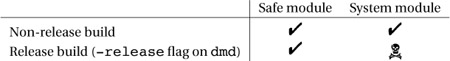
Module safety is orthogonal to choosing a release build for your application. You direct the D compiler to build a release version by passing it a command-line flag (-release in the reference implementation). In a safe module, array bounds are always checked. In a system module, bounds checks are inserted only for non-release builds. In a non-release build, the compiler also inserts other checks such as assert expressions and contract assertions (see Chapter 10 for a thorough discussion of what the release mode entails). The interaction between safe versus system modules and release versus non-release modes is summarized in Table 4.1.

Table 4.1. Presence of bounds checking depending on module kind and build mode

You’ve been warned.

4.1.3 Slicing

Slicing is a powerful feature that allows you to select and work with only a contiguous portion of an array. For example, say you want to print only the last half of an array:

The program above prints

To extract a slice out of array, use the notation array[m .. n], which extracts the portion of the array starting at index m and ending with (and including) index n - 1. The slice has the same type as array itself, so you can, for example, reassign the slice back to the array it originated from:

The symbol $ may participate in an expression inside either limit of the slice and—just as in the case of simple indexing—stands in for the length of the array being sliced. The situation m==n is acceptable and yields an empty slice. However, slices with m > n or n > array.length are illegal. Checking for such illegal cases obeys the bounds checking rules described previously (§ 4.1.2 on page 95).

The expression array[0 .. $] extracts a slice including the entire contents of array. That expression is encountered quite often, so the language gives a hand by making array[] equivalent to array[0 .. $].

4.1.4 Copying

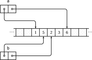
At a minimum, an array object keeps (or can compute in negligible time) two key pieces of information, namely the upper and lower bounds of its data chunk. For example, executing

leads to a state illustrated in Figure 4.1. The array “sees” only the region between its bounds; the hashed area is inaccessible to it.

Figure 4.1. An array object referring to a chunk of five elements.

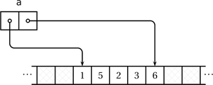
(Other representations are possible, for example, storing the address of the first element and the length of the block, or the address of the first element and the address just past the last element. All representations have access to the same essential information.)

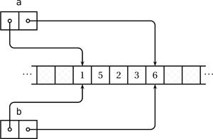
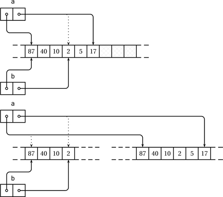
Initializing one array from another (auto b = a;) or assigning one array from another (int[] b; ... b = a;) does not automatically copy data under the hood. Such operations simply make b refer to the same memory chunk as a, as shown in Figure 4.2 on the facing page.

Figure 4.2. Executing auto b = a; does not copy the contents of a but creates a new array object referring to the same chunk of data.

Furthermore, taking a slice off b reduces the chunk “seen” by b, again without copying it. Starting from the state in Figure 4.2 on the next page, if we now execute

then b shrinks in range, again without any data copying (Figure 4.3 on the facing page).

Figure 4.3. Executing b = b[1 .. $ - 2]; shrinks the chunk controlled by b without copying the selected slice.

As a direct consequence of the data sharing illustrated in the figures, writing an element of one array may be reflected in others:

4.1.5 Comparing for Equality

The expression a is b (§ 2.3.4.3 on page 48) compares the bounds of the two arrays for equality and yields true if and only if a and b are bound to the same exact region of memory. No comparison of content is carried out at all.

To compare arrays a and b for element-for-element equality, use a == b or its negation a != b (§ 2.3.12 on page 56).

Comparing for equality iterates in lockstep through all elements of the two arrays and compares them in turn with ==.

4.1.6 Concatenating

The construct

is a concatenation expression. The result of the concatenation is a new array with the contents of lhs followed by the contents of rhs. You may concatenate two arrays of types T[] and T[]; array with value (T[] and T); and value with array (T and T[]).

A concatenation always allocates a new array.

4.1.7 Array-wise Expressions

A few operations apply to arrays as a whole, without any explicit iteration. To create an array-wise expression, specify a trailing [] or [m .. n] on all slices involved in the expression, including the left-hand side of assignments, like this:

An array-wise expression has one of the following forms:

• A single value, such as 5
• A slice explicitly trailed with [] or [m .. n], such as a[] or a[1 .. $ - 1]
• Any valid D expression involving the two terms above, the unary operators - and ~, and the binary operators +, -, *, /, %, ^^, ^, &, |, =, +=, -=, *=, /=, %=, ^=, &=, and |=

The effect of an array-wise expression is that of a loop assigning each element of the left-hand side in turn with the corresponding index of the right-hand side. For example, the assignment

is the same as

Bounds checking rules apply normally according to § 4.1.2 on page 95.

Using slices suffixed with [] or ‘[m .. n]’, numbers, and the allowed operators, you may form parenthesized expressions of any depth and complexity, for example:

One popular use of array-wise operations is simple filling and copying:

Warning

Array-wise operations are powerful, but with great power comes great responsibility. You are responsible for making sure that the lvalue and the rvalue parts of any assignment in an array-wise operation do not overlap. The compiler is free to assume that when optimizing the operations into primitive vector operations offered by the host processor. If you do have overlapping, you’ll need to write the loops by hand, in which case the compiler is not allowed to make any unchecked assumptions.

4.1.8 Shrinking

Array shrinking means that the array should “forget” about some elements from either the left or the right end, without needing to move the rest. The restriction on moving is important; if moving elements were an option, arrays would be easy to shrink—just create a new copy containing the elements to be kept.

Shrinking an array is the easiest thing: just assign to the array a slice of itself.

All shrink operations take time independent of the array’s length (practically they consist only of a couple of word assignments). Affordable shrinking from both ends is a very useful feature of D arrays. (Other languages allow cheap array shrinking from the right, but not from the left because the latter would involve moving over all elements of the array to preserve the location of the array’s left edge.) In D you can take a copy of the array and progressively shrink it to systematically manipulate elements of the array, confident that the constant-time shrinking operations have no significant impact upon the processing time.

For example, let’s write a little program that detects palindrome arrays passed via the command line. A palindrome array is left-right symmetric; for example, [5, 17, 8, 17, 5] is a palindrome, but [5, 7, 8, 7] is not. We need to avail ourselves of a few helpers. One is command line fetching, which nicely comes as an array of strings if you define main as main(string[] args). Then we need to convert arguments from strings to ints, for which we use the function aptly named to in the std.conv module. For some string str, evaluating to!int(str) parses str into an int. Armed with these features, we can write the palindrome test program like this:

First, the program must get rid of the program name from the argument list, which follows a tradition established by C. When you invoke our program (call it “palindrome”) like this:

then the array args contains ["palindrome", "34", "95", "548"]. Here’s where shrinking from the left args = args[1 .. $] comes in handy, reducing args to ["34", "95", "548"]. Then the program iteratively compares the two ends of the array. If they are different, there’s no purpose in continuing to test, so write "no palindrome" and bail out. If the test succeeds, args is reduced simultaneously from its left and right ends. Only if all tests succeed and args got shorter than two elements (the program considers arrays of zero or one element palindromes), the program prints "palindrome" and exits. Although it does a fair amount of array manipulation, the program does not allocate any memory—it just starts with the preallocated array args and shrinks it.

4.1.9 Expanding

On to expanding arrays. To expand an array, use the append operator ‘~=’, for example:

Expanding arrays has a couple of subtleties that concern possible reallocation of the array. Consider:

Does the post-append assignment to a[0] also affect b[0], or, in other words, do a and b still share data post-reallocation? The short answer is, b[0] may or may not be 15—the language makes no guarantee.

Realistically, there is no way to always have enough room at the end of a to reallocate it in place. At least sometimes, reallocation must occur. One easy way out would be to always reallocate a upon appending to it with ~=, there by always making a~=b the same exact thing as a = a ~ b, that is, “Allocate a new array consisting of a concatenated with b and then bind a to that new array.” Although that behavior is easiest to implement, it has serious efficiency problems. For example, oftentimes arrays are iteratively grown in a loop:

For 100 elements, pretty much any expansion scheme would work, but when arrays become larger, only solid solutions can remain reasonably fast. One particularly unsavory approach would be to allow the convenient but inefficient expansion syntax a~=b and encourage it for short arrays but discourage it on large arrays in favor of another, less convenient syntax. At best, the simplest and most intuitive syntax works for short and long arrays.

D leaves ~= the freedom of either expanding by reallocation or opportunistically expanding in place if there is enough unused memory at the end of the current array. The decision belongs entirely to the implementation of ~=, but client code is guaranteed good average performance over a large number of appends to the same array.

Figure 4.4 on the facing page illustrates the two possible outcomes of the expansion request a ~= [5, 17].

Figure 4.4. Two possible outcomes of an attempt to expand array a. In the first case (top), the memory chunk had available memory at its end, which is used for in-place expansion. In the second case, there was no more available room so a new chunk was allocated and a was adjusted to refer to it. Consequently, after expansion, a’s and b’s chunks may or may not overlap.

Depending on how the underlying memory allocator works, an array can expand in more ways than one:

• Often, allocators can allocate chunks only in specific sizes (e.g., powers of 2). It is therefore possible that a request for 700 bytes would receive 1024 bytes of storage, of which 324 are slack. When an expansion request occurs, the array may check whether there’s slack storage and use it.
• If there is no slack space left, the array may initiate a more involved negotiation with the underlying memory allocator. “You know, I’m sitting here and could use some space to the right. Is by any chance the adjacent block available?” The allocator may find an empty block to the right of the current block and gobble it into its own block. This operation is known as coalescing. Then expansion can still proceed without moving any data.
• Finally, if there is absolutely no room in the current block, the array allocates a brand-new block and copies all of its data in it. The implementation may deliberately allocate extra slack space when, for example, it detects repeated expansions of the same array.

An expanding array never stomps on an existing array. For example:

The code above is carefully crafted to fool a into thinking it has room at its end: initially a received a larger size, and then b received the upper part of a and a got reduced to its lower part. Prior to appending to a, the arrays occupy adjacent chunks with a to the left of b. The post-append assert, however, confirms that a actually got reallocated, not expanded in place. The append operator appends in place only when it can prove there is no other array to the right of the expanding one and is always free to conservatively reallocate whenever the slightest suspicion is afoot.

4.1.10 Assigning to .length

Assigning to array.length allows you to either shrink or expand array, depending on the relation of the new length to the old length. For example:

If the array grows as a result of assigning to .length, the added elements are initialized with T.init. The growth strategy and guarantees are identical to those of the append operator ~= (§ 4.1.9 on page 103).

If the array shrinks as a result of assigning to .length, D guarantees the array is not reallocated. Practically, if n <= a.length, a.length = n is equivalent to a = a[0 .. n]. (However, that guarantee does not also imply that further expansions of the array will avoid reallocation.)

You may carry out read-modify-write operations with .length, for example:

Not much magic happens here; all the compiler does is to rewrite array.length ‹op› = b into array.length = array.length ‹op› b. There is some minor magic involved, though (just a sleight of hand, really): array is evaluated only once in the rewritten expression, which is relevant if array is actually some elaborate expression.

4.2 Fixed-Size Arrays

D offers arrays of a size known during compilation, declared, for example, like this:

For each type T and size n, the type T[n] is distinct from any other—for example, uint[10] is distinct from uint[11] and also from int[10].

All fixed-size array values are allocated statically at the place of declaration. If the array value is defined globally, it goes in the per-thread data segment of the program. If allocated inside a function, the array will be allocated on the stack of that function upon the function call. (This means that defining very large arrays in functions may be dangerous.) If, however, you define such an array with static inside a function, the array is allocated in the per-thread data segment so there is no risk of stack overflow.

Upon creation, a fixed-size array T[n] value has all of its data initialized to T.init. For example:

You can initialize a T[n] with a literal:

Beware, however: if you replace int[3] above with auto, a’s type will be deduced as int[], not int[3]. Although it seems logical that the type of [1, 2, 3] should be int[3], which in a way is more “precise” than int[], it turns out that dynamically sized arrays are used much more often than fixed-size arrays, so insisting on fixed-size array literals would have been a usability impediment and a source of unpleasant surprises. Effectively, the use of literals would have prevented the gainful use of auto. As it is, array literals are T[] by default, and T[n] if you ask for that specific type and if n matches the number of values in the literal (as the code above shows).

If you initialize a fixed-size array of type T[n] with a single value of type T, the entire array will be filled with that value:

If you plan to leave the array uninitialized and fill it at runtime, just specify void as an initializer:

Such uninitialized arrays are particularly useful for large arrays that serve as temporary buffers. But beware—an uninitialized integral may not cause too much harm, but uninitialized values of types with indirections (such as multidimensional arrays) are unsafe.

Accessing elements of fixed-size arrays is done by using the indexing operator a[i], the same way as for dynamic arrays. Iteration is also virtually identical to that of dynamic arrays. For example, creating an array of 1024 random numbers would go like this:

The loop could use ref values to use array elements without indexing:

4.2.1 Length

Obviously, fixed-size arrays are aware of their length because it’s stuck in their very type. Unlike dynamic arrays’ length, the .length property is read-only and a static constant. This means you can use array.length for fixed-size arrays whenever a compile-time constant is required, for example, in the length of another fixed-size array definition:

Inside an index expression for array a, $ can be used in lieu of a.length and is, again, a compile-time expression.

4.2.2 Bounds Checking

Bounds checking for fixed-size arrays has an interesting twist. Whenever indexing is used with a compile-time expression, the compiler checks validity during compilation and refuses to compile in case of an out-of-bounds access. For example:

If the expression is a runtime value, compile-time bounds checking is done on a best-effort basis, and runtime checking follows the same protocol as bounds checking for dynamic arrays (§ 4.1.2 on page 95).

4.2.3 Slicing

Taking any slice off an array of type T[n] yields an array of type T[] without an intervening copy:

Compile-time bounds checking is carried out against either or both bounds when they are compile-time constants.

If you take a slice with compile-time-known limits T[a1 .. a2] off an array T[n], and if you request an array of type T[a2 - a1], the compiler grants the request. (The default type yielded by the slice operation—e.g., if you use auto—is still T[].) For example:

4.2.4 Copying and Implicit Conversion

Unlike dynamic arrays, fixed-size arrays have value semantics. This means that copying arrays, passing them into functions, and returning them from functions all copy entire arrays. For example:

Passing entire arrays by value may be inefficient for large arrays, but it has many advantages. One advantage is that short arrays and pass-by-value are frequently used in high-performance computing. Another advantage is that pass-by-value has a simple cure—whenever you want reference semantics, just use ref or automatic conversion to T[] (see the next paragraph). Finally, value semantics makes fixed-size arrays consistent with many other aspects of the language. (Historically, D had reference semantics for fixed-size arrays, which turned out to be a continuous source of contortions and special casing in client code.)

Arrays of type T[n] are implicitly convertible to arrays of type T[]. The dynamic array thus obtained is not allocated anew—it simply latches on to the bounds of the source array. Therefore, the conversion is considered unsafe if the source array is stack-allocated. The implicit conversion makes it easy to pass fixed-size arrays of type T[n] to functions expecting T[]. However, if a function has T[n] as its return type, its result cannot be automatically converted to T[].

You can duplicate a fixed-size array with the .dup property (§ 4.1 on page 93), but you don’t get an object of type T[n] back; you get a dynamically allocated array of type T[] that contains a copy of the fixed-size array. This behavior is sensible given that you otherwise don’t need to duplicate a fixed-size array—to obtain a duplicate of a, just say auto copy = a. With .dup, you get to make a dynamic copy of a fixed-size array.

4.2.5 Comparing for Equality

Fixed-size arrays may be compared with is and ==, just like dynamic arrays (§ 4.1.5 on page 100). You may also transparently mix fixed-size and dynamic-size arrays in comparisons:

4.2.6 Concatenating

Concatenation follows rules similar to those governing concatenation of dynamic arrays (§ 4.1.6 on page 100). There is one important difference. If you ask for a fixed-size array, you get a fixed-size array. Otherwise, you get a newly allocated dynamic array. For example:

Whenever a fixed-array is requested as the result of the concatenating operator ~, there is no dynamic allocation—the result is statically allocated and the result of the concatenation is copied into it.

4.2.7 Array-wise Operations

Array-wise operations on static arrays work similarly to those for dynamic arrays (§ 4.1.7 on page 100). Wherever possible, the compiler performs compile-time bounds checking for arrays bearing static lengths involved in an array-wise expression. You may mix fixed-size and dynamic arrays in expressions.

4.3 Multidimensional Arrays

Since T[] is a dynamic array with elements of type T, and T[] itself is a type, it’s easy to infer that T[][] is an array of T[]s, or, put another way, an array of arrays of Ts. Each element of the outer array is in turn an array offering the usual array primitives. Let’s give T[][] a test drive.

The shape of array defined above is triangular: the first row has five doubles, the second has four, and so on to the fifth one (technically row four), which has one element. Multidimensional arrays obtained by simply composing dynamic arrays are called jagged arrays because their rows may assume arbitrary lengths (as opposed to the somewhat expected straight right edge obtained when all rows have the same length). Figure 4.5 illustrates array’s emplacement in memory.

Figure 4.5. A jagged array storing a triangular matrix as defined in the example on the previous page.

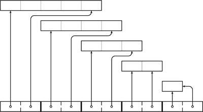
To access an element in a jagged array, specify indices for each dimension in turn; for example, array[3][1] accesses the second element in the fourth row of a jagged array.

Jagged arrays are not contiguous. On the plus side, this means that jagged arrays can spread themselves in memory and require smaller amounts of contiguous memory. The ability to store rows of different lengths may save quite a bit of memory, too. On the minus side, “tall and thin” arrays with many rows and few columns incur a large size overhead as there’s one array to keep per column. For example, one array with 1,000,000 rows each having only 10 integers needs to hold an array of 2,000,000 words (one array per row) plus the management overhead of 1,000,000 small blocks, which, depending on the memory allocator implementation, may be considerable relative to the small perrow payload of 10 ints (40 bytes).

Jagged arrays may have problems with efficiency of access and cache friendliness. Each element access requires two indirections, first through the outer array corresponding to the row, and then through the inner array corresponding to the column. Iterating row-wise is not much of a problem if you first fetch the row and then use it, but going column-wise through a jagged array is a cache miss bonanza.

If the number of columns is known during compilation, you can easily compose a fixed-size array with a dynamic array:

In the example above it is crucial to use ref with foreach. Without ref, the value semantics of double[columns] (§ 4.2.4 on page 109) would create a copy of each row being iterated, which is likely to put a damper on the speed of your code.

If you know the number of both rows and columns during compilation, you may want to use a fixed-size array of fixed-size arrays, as follows:

To access an element at row i and column j, write matrix[i][j]. One small oddity is that the declaration specifies the sizes for each dimension in right-to-left order (i.e., double[columns][rows]), but when accessing elements, indices come in left-to-right order. This is because [] and [n] in types bind right to left, but in expressions they bind left to right.

A variety of multidimensional array shapes can be created by composing fixed-size arrays and dynamic arrays. For example, int[5][][15] is a three-dimensional array consisting of 15 arrays, each being a dynamically allocated array of blocks of five ints each.

4.4 Associative Arrays

An array could be thought of as a function that maps positive integers (indices) to values of some arbitrary type (the data stored in the array). The function is defined only for integers from zero to the array’s length minus one and is entirely tabulated by the contents of the array.

Seen from that angle, associative arrays introduce a certain generalization of arrays. Instead of integers, an associative array may accept an (almost) arbitrary type as its domain. For each value in the domain, it is possible to map a value of a different type—similarly to an array’s slot. The storage method and associated algorithms are different from those of arrays, but, much like an array, an associative array offers fast storage and retrieval of a value given its key.

The type of an associative array is suggestively denoted as V[K], where K is the key type and V is the associated value type. For example, let’s create and initialize an associative array that maps strings to integers:

An associative array literal (introduced in § 2.2.6 on page 39) is a comma-separated list of terms of the form key : value, enclosed in square brackets. In the case above the literal is informative enough to make the explicit type of aa redundant, so it’s more comfortable to write

4.4.1 Length

For an associative array aa, the property aa.length of type size_t yields the number of keys in aa (and also the number of values, given that there is a one-to-one mapping of keys to values). The type of aa.length is size_t.

A default-constructed associative array has length equal to zero and also compares equal to null.

Unlike the homonym property for arrays, associative arrays’ .length is not writable. You may, however, write null to an associative array to clear it.

4.4.2 Reading and Writing Slots

To write a new key/value pair into aa, or to overwrite the value currently stored for that key, just assign to aa[key] like this:

To read a value off an associative array given a key, just read aa[key]. (The compiler distinguishes reads from writes and invokes slightly different functions.) Continuing the example above:

If you try to read the value for a key not found in the associative array, a range violation exception is thrown. Oftentimes, throwing an exception in case a key doesn’t exist is a bit too harsh to be useful, so associative arrays offer a read with a default in the form of a two-argument get method. In the call aa.get(key, defaultValue), if key is found in the map, its corresponding value is returned and defaultValue is not evaluated; otherwise, defaultValue is evaluated and returned as the result of get.

If you want to peacefully test for the existence of a key in an associative array, use the in operator:

4.4.3 Copying

Associative arrays are sheer references with shallow copying: copying or assigning associative arrays just creates new aliases for the same underlying slots. For example:

4.4.4 Comparing for Equality

The operators is, ==, and != work the expected way. For two associative arrays of the same type a and b, the expression a is b yields true if and only if a and b refer to the same associative array (e.g., one was initialized as a copy of the other). The expression a == b compares the key/value pairs of two arrays with == in turn. For a and b to be equal, they must have equal key sets and equal values associated with each key.

4.4.5 Removing Elements

To remove a key/value pair from the map, pass the key to the remove method of the associative array.

The remove method returns a bool that is true if the deleted key was in the associative array, or false otherwise.

4.4.6 Iterating

You can iterate an associative array by using the good old foreach statement (§ 3.7.5 on page 75). The key/value slots are iterated in an unspecified order:

The program above will print

To fetch a copy of all keys in an array, use the .keys property. For an associative array aa of type V[K], the type returned by aa.keys is K[].

Similarly, for aa of type V[K], the aa.values property yields the values stored in aa as an array of type V[]. Generally, it is preferable to iterate with foreach instead of fetching keys of values because the properties allocate a new array, which may be a considerable size for large associative arrays.

Two methods offer iteration through the keys and the values of an associative array without creating new arrays: aa.byKey() spans only the keys of the associative array aa, and aa.byValue() spans the values. For example:

4.4.7 User-Defined Types as Keys

Internally, associative arrays use hashing and sorting for keys to ensure fast retrieval of values given keys. For a user-defined type to be used as a key in an associative array, it must define two special methods, opHash and opCmp. We haven’t yet learned how to define user-defined types and methods, so for now let’s defer that discussion to Chapter 6.

4.5 Strings

Strings receive special treatment in D. Two decisions made early in the definition of the language turned out to be winning bets. First, D embraces Unicode as its standard character set. Unicode is today’s most popular and comprehensive standard for defining and representing textual data. Second, D chose UTF-8, UTF-16, and UTF-32 as its native encodings, without favoring any and without preventing your code from using other encodings.

In order to understand how D deals with text, we need to acquire some knowledge of Unicode and UTF. For an in-depth treatment, Unicode Explained [36] is a useful resource; the Unicode Consortium Standard document, currently in the fifth edition corresponding to version 5.1 of the Unicode standard [56], is the ultimate reference.

4.5.1 Code Points

One important fact about Unicode that, once understood, dissipates a lot of potential confusion is that Unicode separates the notion of abstract character, or code point, from the notion of representation, or encoding. This is a nontrivial distinction that often escapes the unwary, particularly because the well-known ASCII standard has no notion of separate representation. Good old ASCII maps each character commonly used in English text, plus a few “control codes,” to a number between 0 and 127—that is, 7 bits. Since at the time ASCII got introduced most computers already used the 8-bit byte (octet) as a unit of addressing, there was no question about “encoding” ASCII text at all: use 7 bits off an octet; that was the encoding. (The remaining bit left the door open for creative uses, which led to a Cambrian explosion of mutually incompatible extensions.)

Unicode, in contrast, first defines code points, which are, simply put, numbers assigned to abstract characters. The abstract character “A” receives number 65, the abstract character € receives number 8364, and so on. Deciding which symbols deserve a place in the Unicode mapping and how to assign numbers to them is one important task of the Unicode Consortium, and that’s great because the rest of us can use the mapping without worrying about the minutiae of defining and documenting it.

As of version 5.1, Unicode code points lie between 0 and 1,114,111 (the upper limit is more often expressed in hexadecimal: 0x10FFFF or, in Unicode’s specific spelling, U+10FFFF). A common misconception about Unicode is that 2 bytes are enough to represent any Unicode character, perhaps because some languages standardized on 2-byte characters originating in earlier versions of the Unicode standard. In fact, there are exactly 17 times more Unicode symbols than the 65,536 afforded by a 2-byte representation. (Truth be told, most of the higher code points are seldom used or not yet allocated.)

Anyhow, when discussing code points, representation should not necessarily come to mind. At the highest level, code points are a giant tabulated function mapping integers from 0 to 1,114,111 to abstract character entities. There are many details on how that numeric range is allocated, but that does not diminish the correctness of our highest-level description. Exactly how to put Unicode code points in sequences of bytes is something that encodings need to worry about.

4.5.2 Encodings

If Unicode simply followed ASCII’s grand tradition, it would have just rounded the upper limit 0x10FFFF to the next byte, obtaining a simple 3-byte representation for each code point. This potential representation has an issue, however. Most text in English or other Latin-derived writing systems would use a statistically very narrow range of code points (numbers), which leads to wasted space. The storage for the typical Latin text would just blow up in size by a factor of three. Richer alphabets such as Asian writing systems would make better use of the three bytes, and that’s fine because there would be fewer total symbols in the text (each symbol is more informative).

To address the issue of wasting space, Unicode adopted several variable-length encoding schemes. Such schemes use one or more narrow codes to represent the full range of Unicode code points. The narrow codes (usually 8- or 16-bit) are known as code units. Each code point is represented by one or more code units.

UTF-8 is the first encoding that was standardized. UTF-8, invented by Ken Thompson in one evening inside a New Jersey diner [47], is an almost canonical example of solid, ingenious design. The basic idea behind UTF-8 is to use 1 to 6 bytes for encoding any given character, and to add control bits to disambiguate between encodings of different lengths. UTF-8 is identical to ASCII for the first 127 code points. That instantly makes any ASCII text also valid UTF-8 text, which in and of itself was a brilliant move. For code points beyond the ASCII range, UTF-8 uses a variable-length encoding, shown in Table 4.2.

Table 4.2. UTF-8 encodings. The choice of control bits allows midstream synchronization, error recovery, and backward iteration.

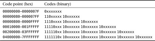
Since today the range of defined Unicode code points stops at 0x10FFFF, the last two sequences are reserved for future use; only up to 4-byte encodings are currently valid.

The control bit patterns chosen have two interesting properties:

1. A non-leading byte is never equal to a leading byte.
2. The first byte unambiguously determines the length of an encoding.

The first property is crucial because it enables two important applications. One is simple synchronization—if you pick up a UTF-8 transmission somewhere in midstream, you can easily figure out where the next code point starts: just look for the next byte with anything but 10 as its most significant bits. The other application is backward iteration—it is easy to go backward in a UTF-8 string without ever getting confused. Backward iteration opens UTF-8 strings to a host of algorithms (e.g., finding the last occurrence of a string in another can be implemented efficiently). The second property is not essential but simplifies and accelerates string processing.

Ideally, frequent code points should have small values and infrequent ones should have large values. If that condition is fulfilled, UTF-8 acts as a good statistical encoder by encoding more frequent symbols in fewer bits. This is certainly the case for Latin-derived languages, where most code units fit in 1 byte and the occasional accented characters fit in 2.

UTF-16 is also a variable-length encoding but uses a different (and arguably less elegant) approach to encoding. Code points between 0 and 0xFFFF are encoded as a sole 16-bit code unit and code points between 0x10000 and 0x10FFFF are represented by a pair in which the first code unit is in the range 0xD800 through 0xDBFF and the second code unit is in the range 0xDC00 through 0xDFFF. To support this encoding, Unicode allocates no valid characters to numbers in the range 0xD800 through 0xDBFF. The two ranges are called high surrogate area and low surrogate area, respectively.

One criticism commonly leveled against UTF-16 is that it makes the statistically rare cases also the most complicated and the ones deserving the most scrutiny. Most—but alas, not all—Unicode characters (the so-called Basic Multilingual Plane) do fit in one UTF-16 code unit, and therefore a lot of UTF-16 code tacitly assumes one code unit per character and is effectively untested for surrogate pairs. To further the confusion, some languages initially centered their string support around UCS-2, a precursor of UTF-16 with exactly 16 bits per code point, to later add UTF-16 support, subtly obsoleting older code that relied on a one-to-one mapping between characters and codes.

Finally, UTF-32 uses 32 bits per code unit, which allows a true one-to-one mapping of code points to code units. This means UTF-32 is the simplest and easiest-to-use representation, but it’s also the most space-consuming. A common recommendation is to use UTF-8 for storage and UTF-32 temporarily during processing if necessary.

4.5.3 Character Types

D defines three character types: char, wchar, and dchar, representing code units for UTF-8, UTF-16, and UTF-32, respectively. Their .init values are intentionally invalid encodings: char.init is 0xFF, wchar.init is 0xFFFF, and dchar.init is 0x0000FFFF. Table 4.2 on page 119 clarifies that 0xFF may not be part of any valid UTF-8 encoding, and also Unicode deliberately assigns no valid code point for 0xFFFF.

Used individually, the three character types mostly behave like unsigned integers and can occasionally be used to store invalid UTF code points (the compiler does not enforce valid encodings throughout), but the intended meaning of char, wchar, and dchar is as UTF code points. For general 8-, 16-, and 32-bit unsigned integers, or for using encodings other than UTF, it’s best to use ubyte, ushort, and uint, respectively. For example, if you want to use pre-Unicode 8-bit code pages, you may want to use ubyte, not char, as your building block.

4.5.4 Arrays of Characters + Benefits = Strings

When assembling any of the character types in an array—as in char[], wchar[], or dchar[]—the compiler and the runtime support library “understand” that you are working with UTF-encoded Unicode strings. Consequently, arrays of characters enjoy the power and versatility of general arrays, plus a few extra goodies as Unicode denizens.

In fact, D already defines three string types corresponding to the three character widths: string, wstring, and dstring. They are not special types at all; in fact, they are aliases for character array types, with a twist: the character type is adorned with the immutable qualifier to disallow arbitrary changes of individual characters in strings. For example, type string is a synonym for the more verbose type immutable(char)[]. We won’t get to discussing type qualifiers such as immutable until Chapter 8, but for strings of all widths the effect of immutable is very simple: a string, aka an immutable(char)[], is just like a char[] (and a wstring is just like a wchar[], etc.), except you can’t assign new values to individual characters in the string:

To change one individual character in a string, you need to create another string via concatenation:

Why such a decision? After all, in the case above it’s quite a waste to allocate a whole new string (recall from § 4.1.6 on page 100 that ~ always allocates a new array) instead of just modifying the existing one. There are, however, a few good reasons for disallowing modification of individual characters in strings. One reason is that immutable simplifies situations when string, wstring, and dstring objects are copied and then changed. Effectively immutable ensures no undue aliasing between strings. Consider:

With immutable characters, you know you can have several variables refer to the same string, without fearing that modifying one would also modify the others. Copying string objects is very cheap because it doesn’t need to do any special copy management (such as eager copy or copy-on-write).

An equally strong reason for disallowing changes in strings at code unit level is that such changes don’t make much sense anyway. Elements of a string are variable-length, and most of the time you want to replace logical characters (code points), not physical chars (code units), so you seldom want to do surgery on individual chars. It’s much easier to write correct UTF code if you forgo individual char assignments and you focus instead on manipulating entire strings and fragments thereof. D’s standard library sets the tone by fostering manipulation of strings as whole entities instead of focusing on indices and individual characters. However, UTF code is not trivially easy to write; for example, the concatenation 'H' ~ a[1 .. $] above has a bug in the general case because it assumes that the first code point in a has exactly 1 byte. The correct way to go about it is

The function stride, found in the standard library module std.utf, returns the length of the code starting at a specified position in a string. (To use stride and related library artifacts, insert the line

near the top of your program.) In our case, the call stride(a, 0) returns the length of the encoding for the first character (aka code point) in a, which we pass to select the offset marking the beginning of the second character.

A very visible artifact of the language’s support for Unicode can be found in string literals, which we’ve already looked at (§ 2.2.5 on page 35). D string literals understand Unicode code points and automatically encode them appropriately for whichever encoding scheme you choose. For example:

Although the internal representations of a, b, and c are very different, you don’t need to worry about that because you express the literal in an abstract way by using code points. The compiler takes care of all encoding details, such that in the end the program prints three lines containing the same exact text:

The encoding of the literal is determined by the context in which the literal occurs. In the cases above, the compiler has the literal morph without any runtime processing into the encodings UTF-8, UTF-16, and UTF-32 (corresponding to types string, wstring, and dstring), in spite of it being spelled the exact same way throughout. If the requested literal encoding is ambiguous, suffixing the literal with one of c, w, or d (something "like that"d) forces the encoding of the string to UTF-8, UTF-16, and UTF-32, respectively (refer to § 2.2.5.2 on page 37).

4.5.4.1 foreach with Strings

If you iterate a string str of any width like this:

then c will iterate every code unit of str. For example, if str is an array of char (immutable or not), c takes type char. This is expected from the general behavior of foreach with arrays but is sometimes undesirable for strings. For example, let’s print each character of a string enclosed in square brackets:

The program above ungainly prints

The reverse video ? (which may vary depending on system and font used) is the console’s mute way of protesting against seeing an invalid UTF code. Of course, trying to print alone a char that would make sense only in combination with other chars is bound to fail.

The interesting part starts when you specify a different character type for c. For example, specify dchar for c:

In this case, the compiler automatically inserts code for transcoding on the fly each code unit in str in the representation dictated by c’s type. The loop above prints

which indicates that the double-byte characters å and ä were converted correctly to one dchar each and subsequently printed correctly. The same exact result would be printed if c had type wchar because the two non-ASCII characters used fit in one UTF-16 unit each, but not in the most general case (surrogate pairs would be wrongly processed). To be on the safe side, it is of course best to use dchar with loops over strings.

In the case above, the transcoding performed by foreach went from a narrow to a wide representation, but it could go either way. For example, you could start with a dstring and iterate it one (encoded) char at a time.

4.6 Arrays’ Maverick Cousin: The Pointer

An array object tracks a chunk of typed objects in memory by storing the lower and upper bound. A pointer is “half” an array—it tracks only one object. As such, the pointer does not have information on whether the chunk starts and ends. If you have that information from the outside, you can use it to move the pointer around and make it point to neighboring elements.

A pointer to an object of type T is denoted as type T*, with the default value null (i.e., a pointer that points to no actual object). To make a pointer point to an object, use the address-of operator &, and to use that object, use the dereference operator * (§ 2.3.6.2 on page 52). For example:

Pointers allow arithmetic that makes them apt as cursors inside arrays. Incrementing a pointer makes it point to the next element of the array; decrementing it moves it to the previous element. Adding an integer n to a pointer yields a pointer to an object situated n positions away in the array, to the right if n is positive and to the left if n is negative. To simplify indexed operations, p[n] is equivalent to *(p + n). Finally, taking the difference between two pointers p2 - p1 yields an integral n such that p1 + n==p2.

You can fetch the address of the first element of an array with a.ptr. It follows that a pointer to the last element of a non-empty array arr can be obtained with arr.ptr + arr.length - 1, and a pointer just past the last element with arr.ptr + arr.length. To exemplify all of the above:

Careful, however: unless you have access to array bounds information from outside the pointer, things could go awry very easily. All pointer operations go completely unchecked—the implementation of the pointer is just a word-long memory address and the corresponding arithmetic just blindly does what you ask. That makes pointers blazingly fast and also appallingly ignorant. Pointers aren’t even smart enough to realize they are pointing at individual objects (as opposed to pointing inside arrays):

Pointers also don’t know when they fall off the limits of arrays:

Writing through a pointer that doesn’t point to valid data is essentially playing Russian roulette with your program’s integrity: the writes could land anywhere, stomping the most carefully maintained data or possibly even code. Such operations make pointers a memory-unsafe feature.

For these reasons, you should consistently avoid pointers and prefer using arrays, class references (Chapter 6), ref function parameters (§ 5.2.1 on page 135), and automatic memory management. All of these are safe, can be effectively checked, and do not undergo significant efficiency loss in most cases.

In fact, arrays are a very useful abstraction, and they were very carefully designed to hit a narrow target: the fastest thing beyond pointers that can be made memory-safe. Clearly a bald pointer does not have access to enough information to figure out anything on its own; arrays, on the other hand, are aware of their extent so they can cheaply verify that all operations are within range.

From a high-level perspective, it could be argued that arrays are rather low-level and that they could have aimed at implementing an abstract data type. On the contrary, from a low-level perspective, it could be argued that arrays are unnecessary because they can be implemented by using pointers. The answer to both arguments is a resounding “Let me explain.”

Arrays are needed as the lowest-level abstraction that is still safe. If only pointers were provided, the language would have been unable to provide any kind of guarantee regarding various higher-level user-defined constructs built on top of pointers. Arrays also should not be a too-high-level feature because they are built in, so everything else comes on top of them. A good built-in facility is low-level and fast such that high-level and perhaps not-as-fast abstractions can be built on top of it. Abstraction never flows the other way.

D offers a proper subset known as SafeD (Chapter 11), and compilers offer a switch that enforces use of that subset. Naturally, most pointer operations are not allowed in SafeD. Built-in arrays are an important enabler of powerful, expressive SafeD programs.

4.7 Summary and Quick Reference

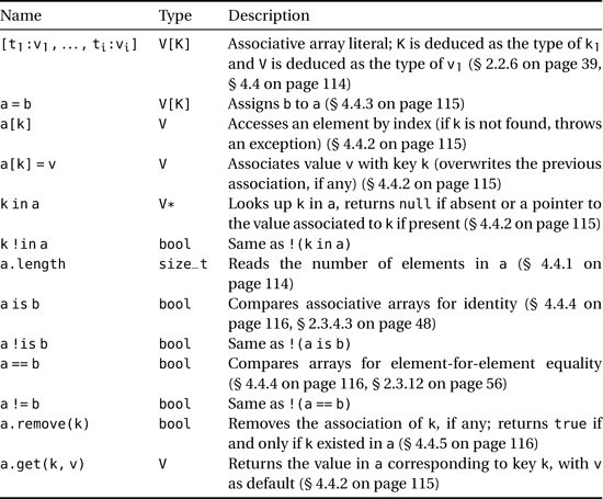
Table 4.3 on the facing page summarizes dynamic array operations; Table 4.4 on page 128 summarizes operations on fixed-size arrays; and Table 4.5 on page 129 summarizes operations available for associative arrays.

Table 4.3. Dynamic array operations (a and b are two values of type T[], t, t₁, ..., t_k are values of type T, and n is a value convertible to type size_t)

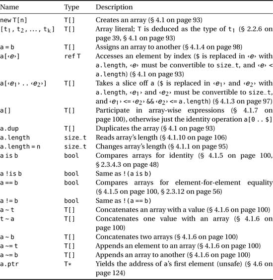
Table 4.4. Fixed-size array operations (a and b are two values of type T[], t, t₁, ..., tk are values of type T, and n is a statically known value convertible to type size_t)

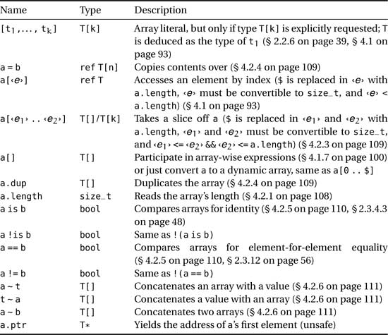
Table 4.5. Associative array operations (a and b are two values of type V[K], k, k₁, ..., k_i are values of type K, and v, v₁, ..., v_k are values of type V)