
Chapter 16
Insurance
We bring together concepts from nearly all the previous chapters to build a DW/BI system for a property and casualty insurance company in this final case study. If you are from the insurance industry and jumped directly to this chapter for a quick fix, please accept our apology, but this material depends heavily on ideas from the earlier chapters. You'll need to turn back to the beginning of the book to have this chapter make any sense.
As has been our standard procedure, this chapter launches with background information for a business case. While the requirements unfold, we'll draft the enterprise data warehouse bus matrix, much like we would in a real-life requirements analysis effort. We'll then design a series of dimensional models by overlaying the core techniques learned thus far.
Chapter 16 reviews the following concepts:
- Requirements-driven approach to dimensional design
- Value chain implications, along with an example bus matrix snippet for an insurance company
- Complementary transaction, periodic snapshot, and accumulating snapshot schemas
- Dimension role playing
- Handling of slowly changing dimension attributes
- Mini-dimensions for dealing with large, rapidly changing dimension attributes
- Multivalued dimension attributes
- Degenerate dimensions for operational control numbers
- Audit dimensions to track data lineage
- Heterogeneous supertypes and subtypes to handle products with varied attributes and facts
- Junk dimensions for miscellaneous indicators
- Conformed dimensions and facts
- Consolidated fact tables combining metrics from separate business processes
- Factless fact tables
- Common mistakes to avoid when designing dimensional models
Insurance Case Study
Imagine working for a large property and casualty insurer that offers automobile, homeowner, and personal property insurance. You conduct extensive interviews with business representatives and senior management from the claims, field operations, underwriting, finance, and marketing departments. Based on these interviews, you learn the industry is in a state of flux. Nontraditional players are leveraging alternative channels. Meanwhile, the industry is consolidating due to globalization, deregulation, and demutualization challenges. Markets are changing, along with customer needs. Numerous interviewees tell us information is becoming an even more important strategic asset. Regardless of the functional area, there is a strong desire to use information more effectively to identify opportunities more quickly and respond most appropriately.
The good news is that internal systems and processes already capture the bulk of the data required. Most insurance companies generate tons of nitty-gritty operational data. The bad news is the data is not integrated. Over the years, political and IT boundaries have encouraged the construction of tall barriers around isolated islands of data. There are multiple disparate sources for information about the company's products, customers, and distribution channels. In the legacy operational systems, the same policyholder may be identified several times in separate automobile, home, and personal property applications. Traditionally, this segmented approach to data was acceptable because the different lines of business functioned largely autonomously; there was little interest in sharing data for cross-selling and collaboration in the past. Now within our case study, business management is attempting to better leverage this enormous amount of inconsistent and somewhat redundant data.
Besides the inherent issues surrounding data integration, business users lack the ability to access data easily when needed. In an attempt to address this shortcoming, several groups within the case study company rallied their own resources and hired consultants to solve their individual short-term data needs. In many cases, the same data was extracted from the same source systems to be accessed by separate organizations without any strategic overall information delivery strategy.
It didn't take long to recognize the negative ramifications associated with separate analytic data repositories because performance results presented at executive meetings differed depending on the data source. Management understood this independent route was not viable as a long-term solution because of the lack of integration, large volumes of redundant data, and difficulty in interpreting and reconciling the results. Given the importance of information in this brave new insurance world, management was motivated to deal with the cost implications surrounding the development, support, and analytic inefficiencies of these supposed data warehouses that merely proliferated operational data islands.
Senior management chartered the chief information officer (CIO) with the responsibility and authority to break down the historical data silos to “achieve information nirvana.” They charged the CIO with the fiduciary responsibility to manage and leverage the organization's information assets more effectively. The CIO developed an overall vision that wed an enterprise strategy for dealing with massive amounts of data with a response to the immediate need to become an information-rich organization. In the meantime, an enterprise DW/BI team was created to begin designing and implementing the vision.
Senior management has been preaching about a transformation to a more customer-centric focus, instead of the traditional product-centric approach, in an effort to gain competitive advantage. The CIO jumped on that bandwagon as a catalyst for change. The folks in the trenches have pledged intent to share data rather than squirreling it away for a single purpose. There is a strong desire for everyone to have a common understanding of the state of the business. They're clamoring to get rid of the isolated pockets of data while ensuring they have access to detail and summary data at both the enterprise and line-of-business levels.
Insurance Value Chain
The primary value chain of an insurance company is seemingly short and simple. The core processes are to issue policies, collect premium payments, and process claims. The organization is interested in better understanding the metrics spawned by each of these events. Users want to analyze detailed transactions relating to the formulation of policies, as well as transactions generated by claims processing. They want to measure performance over time by coverage, covered item, policyholder, and sales distribution channel characteristics. Although some users are interested in the enterprise perspective, others want to analyze the heterogeneous nature of the insurance company's individual lines of business.
Obviously, an insurance company is engaged in many other external processes, such as the investment of premium payments or compensation of contract agents, as well as a host of internally focused activities, such as human resources, finance, and purchasing. For now, we will focus on the core business related to policies and claims.
The insurance value chain begins with a variety of policy transactions. Based on your current understanding of the requirements and underlying data, you opt to handle all the transactions impacting a policy as a single business process (and fact table). If this perspective is too simplistic to accommodate the metrics, dimensionality, or analytics required, you should handle the transaction activities as separate fact tables, such as quoting, rating, and underwriting. As discussed in Chapter 5: Procurement, there are trade-offs between creating separate fact tables for each natural cluster of transaction types versus lumping the transactions into a single fact table.
There is also a need to better understand the premium revenue associated with each policy on a monthly basis. This will be key input into the overall profit picture. The insurance business is very transaction intensive, but the transactions themselves do not represent little pieces of revenue, as is the case with retail or manufacturing sales. You cannot merely add up policy transactions to determine the revenue amount. The picture is further complicated in insurance because customers pay in advance for services. This same advance-payment model applies to organizations offering magazine subscriptions or extended warranty contracts. Premium payments must be spread across multiple periods because the company earns the revenue over time as it provides insurance coverage. The complex relationship between policy transactions and revenue measurements often makes it impossible to answer revenue questions by crawling through the individual transactions. Not only is such crawling time-consuming, but also the logic required to interpret the effect of different transaction types on revenue can be horrendously complicated. The natural conflict between the detailed transaction view and the snapshot perspective almost always requires building both kinds of fact tables in the warehouse. In this case, the premium snapshot is not merely a summarization of the policy transactions; it is quite a separate thing that comes from a separate source.
Draft Bus Matrix
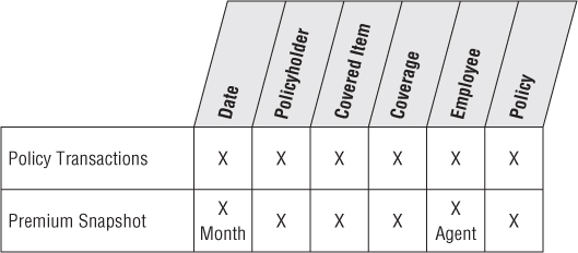
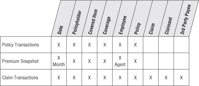
Based on the interview findings, along with an understanding of the key source systems, the team begins to draft an enterprise data warehouse bus matrix with the core policy-centric business processes as rows and core dimensions as columns. Two rows are defined in the matrix, one corresponding to the policy transactions and another for the monthly premium snapshot.
As illustrated in Figure 16.1, the core dimensions include date, policyholder, employee, coverage, covered item, and policy. When drafting the matrix, don't attempt to include all the dimensions. Instead, try to focus on the core common dimensions that are reused in more than one schema.
Figure 16.1 Initial draft bus matrix.
Policy Transactions
Let's turn our attention to the first row of the matrix by focusing on the transactions for creating and altering a policy. Assume the policy represents a set of coverages sold to the policyholder. Coverages can be considered the insurance company's products. Homeowner coverages include fire, flood, theft, and personal liability; automobile coverages include comprehensive, collision damage, uninsured motorist, and personal liability. In a property and casualty insurance company, coverages apply to a specific covered item, such as a particular house or car. Both the coverage and covered item are carefully identified in the policy. A particular covered item usually has several coverages listed in the policy.
Agents sell policies to policyholders. Before the policy can be created, a pricing actuary determines the premium rate that will be charged given the specific coverages, covered items, and qualifications of the policyholder. An underwriter, who takes ultimate responsibility for doing business with the policyholder, makes the final approval.
The operational policy transaction system captures the following types of transactions:
- Create policy, alter policy, or cancel policy (with reason)
- Create coverage on covered item, alter coverage, or cancel coverage (with reason)
- Rate coverage or decline to rate coverage (with reason)
- Underwrite policy or decline to underwrite policy (with reason)
The grain of the policy transaction fact table should be one row for each individual policy transaction. Each atomic transaction should be embellished with as much context as possible to create a complete dimensional description of the transaction. The dimensions associated with the policy transaction business process include the transaction date, effective date, policyholder, employee, coverage, covered item, policy number, and policy transaction type. Now let's further discuss the dimensions in this schema while taking the opportunity to reinforce concepts from earlier chapters.
Dimension Role Playing
There are two dates associated with each policy transaction. The policy transaction date is the date when the transaction was entered into the operational system, whereas the policy transaction effective date is when the transaction legally takes effect. These two foreign keys in the fact table should be uniquely named. The two independent dimensions associated with these keys are implemented using a single physical date table. Multiple logically distinct tables are then presented to the user through views with unique column names, as described originally in Chapter 6: Order Management.
Slowly Changing Dimensions
Insurance companies typically are very interested in tracking changes to dimensions over time. You can apply the three basic techniques for handling slowly changing dimension (SCD) attributes to the policyholder dimension, as introduced in Chapter 5.
With the type 1 technique, you simply overwrite the dimension attribute's prior value. This is the simplest approach to dealing with attribute changes because the attributes always represent the most current descriptors. For example, perhaps the business agrees to handle changes to the policyholder's date of birth as a type 1 change based on the assumption that any changes to this attribute are intended as corrections. In this manner, all fact table history for this policyholder appears to have always been associated with the updated date of birth.
Because the policyholder's ZIP code is key input to the insurer's pricing and risk algorithms, users are very interested in tracking ZIP code changes, so the type 2 technique is used for this attribute. Type 2 is the most common SCD technique when there's a requirement for accurate change tracking over time. In this case, when the ZIP code changes, you create a new policyholder dimension row with a new surrogate key and updated geographic attributes. Do not go back and revisit the fact table. Historical fact table rows, prior to the ZIP code change, still reflect the old surrogate key. Going forward, you use the policyholder's new surrogate key, so new fact table rows join to the post-change dimension profile. Although this technique is extremely graceful and powerful, it places more burdens on ETL processing. Also, the number of rows in the dimension table grows with each type 2 SCD change. Given there might already be more than 1 million rows in your policyholder dimension table, you may opt to use a mini-dimension for tracking ZIP code changes, which we will review shortly.
Finally, let's assume each policyholder is classified as belonging to a particular segment. Perhaps nonresidential policyholders were historically categorized as either commercial or government entities. Going forward, the business users want more detailed classifications to differentiate between large multinational, middle market, and small business commercial customers, in addition to nonprofit organizations and governmental agencies. For a period of time, users want the ability to analyze results by either the historical or new segment classifications. In this case you could use a type 3 approach to track the change for a period of time by adding a column, labeled Historical for differentiation, to retain the old classifications. The new classification values would populate the segment attribute that has been a permanent fixture on the policyholder dimension. This approach, although not extremely common, allows you to see performance by either the current or historical segment maps. This is useful when there's been an en masse change, such as the customer classification realignment. Obviously, the type 3 technique becomes overly complex if you need to track more than one version of the historical map or before-and-after changes for multiple dimension attributes.
Mini-Dimensions for Large or Rapidly Changing Dimensions
As mentioned earlier, the policyholder dimension qualifies as a large dimension with more than 1 million rows. It is often important to accurately track content values for a subset of attributes. For example, you need an accurate description of some policyholder and covered item attributes at the time the policy was created, as well as at the time of any adjustment or claim. As discussed in Chapter 5, the practical way to track changing attributes in large dimensions is to split the closely monitored, more rapidly changing attributes into one or more type 4 mini-dimensions directly linked to the fact table with a separate surrogate key. The use of mini-dimensions has an impact on the efficiency of attribute browsing because users typically want to browse and constrain on these changeable attributes. If all possible combinations of the attribute values in the mini-dimension have been created, handling a mini-dimension change simply means placing a different key in the fact table row from a certain point in time forward. Nothing else needs to be changed or added to the database.
The covered item is the house, car, or other specific insured item. The covered item dimension contains one row for each actual covered item. The covered item dimension is usually somewhat larger than the policyholder dimension, so it's another good place to consider deploying a mini-dimension. You do not want to capture the variable descriptions of the physical covered objects as facts because most are textual and are not numeric or continuously valued. You should make every effort to put textual attributes into dimension tables because they are the target of textual constraints and the source of report labels.
Multivalued Dimension Attributes
We discussed multivalued dimension attributes when we associated multiple skills with an employee in Chapter 9: Human Resources Management. In Chapter 10: Financial Services, we associated multiple customers with an account, and then in Chapter 14: Healthcare, we modeled a patient's multiple diagnoses. In this case study, you'll look at another multivalued modeling situation: the relationship between commercial customers and their industry classifications.
Each commercial customer may be associated with one or more Standard Industry Classification (SIC) or North American Industry Classification System (NAICS) codes. A large, diversified commercial customer could be represented by a dozen or more classification codes. Much like you did with Chapter 14's diagnosis group, a bridge table ties together all the industry classification codes within a group. This industry classification bridge table joins directly to either the fact table or the customer dimension as an outrigger. It enables you to report fact table metrics by any industry classification. If the commercial customer's industry breakdown is proportionally identified, such as 50 percent agricultural services, 30 percent dairy products, and 20 percent oil and gas drilling, a weighting factor should be included on each bridge table row. To handle the case in which no valid industry code is associated with a given customer, you simply create a special bridge table row that represents Unknown.
Numeric Attributes as Facts or Dimensions
Let's move on to the coverage dimension. Large insurance companies have dozens or even hundreds of separate coverage products available to sell for a given type of covered item. The actual appraised value of a specific covered item, like someone's house, is a continuously valued numeric quantity that can even vary for a given item over time, so treat it as a legitimate fact. In the dimension table, you could store a more descriptive value range, such as $250,000 to $299,999 Appraised Value, for grouping and filtering. The basic coverage limit is likely to be more standardized and not continuously valued, like Replacement Value or Up to $250,000. In this case, it would also be treated as a dimension attribute.
Degenerate Dimension
The policy number will be handled as a degenerate dimension if you have extracted all the policy header information into other dimensions. You obviously want to avoid creating a policy transaction fact table with just a small number of keys while embedding all the descriptive details (including the policyholder, dates, and coverages) in an overloaded policy dimension. In some cases, there may be one or two attributes that still belong to the policy and not to another dimension. For example, if the underwriter establishes an overall risk grade for the policy based on the totality of the coverages and covered items, then this risk grade probably belongs in a policy dimension. Of course, then the policy number is no longer a degenerate dimension.
Low Cardinality Dimension Tables
The policy transaction type dimension is a small dimension for the transaction types listed earlier with reason descriptions. A transaction type dimension might contain less than 50 rows. Even though this table is both narrow in terms of the number of columns and shallow in terms of the number of rows, the attributes should still be handled in a dimension table; if the textual characteristics are used for query filtering or report labeling, then they belong in a dimension.
Audit Dimension
You have the option to associate ETL process metadata with transaction fact rows by including a key that links to an audit dimension row created by the extract process. As discussed in Chapter 6, each audit dimension row describes the data lineage of the fact row, including the time of the extract, source table, and extract software version.
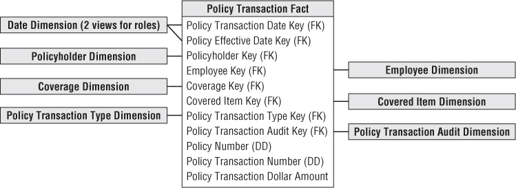
Policy Transaction Fact Table
The policy transaction fact table in Figure 16.2 illustrates several characteristics of a classic transaction grain fact table. First, the fact table consists almost entirely of keys. Transaction schemas enable you to analyze behavior in extreme detail. As you descend to lower granularity with atomic data, the fact table naturally sprouts more dimensionality. In this case, the fact table has a single numeric fact; interpretation of the fact depends on the corresponding transaction type dimension. Because there are different kinds of transactions in the same fact table, in this scenario, you cannot label the fact more specifically.
Figure 16.2 Policy transaction schema.
Heterogeneous Supertype and Subtype Products
Although there is strong support for an enterprise-wide perspective at our insurance company, the business users don't want to lose sight of their line-of-business specifics. Insurance companies typically are involved in multiple, very different lines of business. For example, the detailed parameters of homeowners' coverages differ significantly from automobile coverages. And these both differ substantially from personal property coverage, general liability coverage, and other types of insurance. Although all coverages can be coded into the generic structures used so far in this chapter, insurance companies want to track numerous specific attributes that make sense only for a particular coverage and covered item. You can generalize the initial schema developed in Figure 16.2 by using the supertype and subtype technique discussed in Chapter 10.
Figure 16.3 shows a schema to handle the specific attributes that describe automobiles and their coverages. For each line of business (or coverage type), subtype dimension tables for both the covered item and associated coverage are created. When a BI application needs the specific attributes of a single coverage type, it uses the appropriate subtype dimension tables.
Figure 16.3 Policy transaction schema with subtype automobile dimension tables.
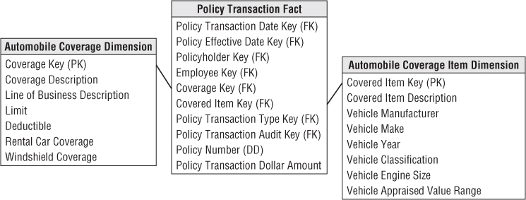
Notice in this schema that you don't need separate line-of-business fact tables because the metrics don't vary by business, but you'd likely put a view on the supertype fact table to present only rows for a given subtype. The subtype dimension tables are introduced to handle the special line-of-business attributes. No new keys need to be generated; logically, all we are doing is extending existing dimension rows.
Complementary Policy Accumulating Snapshot
Finally, before leaving policy transactions, you should consider the use of an accumulating snapshot to capture the cumulative effect of the transactions. In this scenario, the grain of the fact table likely would be one row for each coverage and covered item on a policy. You can envision including policy-centric dates, such as quoted, rated, underwritten, effective, renewed, and expired. Likewise, multiple employee roles could be included on the fact table for the agent and underwriter. Many of the other dimensions discussed would be applicable to this schema, with the exception of the transaction type dimension. The accumulating snapshot likely would have an expanded fact set.
As discussed in Chapter 4: Inventory, an accumulating snapshot is effective for representing information about a pipeline process's key milestones. It captures the cumulative lifespan of a policy, covered items, and coverages; however, it does not store information about each and every transaction that occurred. Unusual transactional events or unexpected outliers from the standard pipeline would likely be masked with an accumulating perspective. On the other hand, an accumulating snapshot, sourced from the transactions, provides a clear picture of the durations or lag times between key process events.
Premium Periodic Snapshot
The policy transaction schema is useful for answering a wide range of questions. However, the blizzard of transactions makes it difficult to quickly determine the status or financial value of an in-force policy at a given point in time. Even if all the necessary detail lies in the transaction data, a snapshot perspective would require rolling the transactions forward from the beginning of history taking into account complicated business rules for when earned revenue is recognized. Not only is this nearly impractical on a single policy, but it is ridiculous to think about generating summary top line views of key performance metrics in this manner.
The answer to this dilemma is to create a separate fact table that operates as a companion to the policy transaction table. In this case, the business process is the monthly policy premium snapshot. The granularity of the fact table is one row per coverage and covered item on a policy each month.
Conformed Dimensions
Of course, when designing the premium periodic snapshot table, you should strive to reuse as many dimensions from the policy transaction table as possible. Hopefully, you have become a conformed dimension enthusiast by now. As described in Chapter 4, conformed dimensions used in separate fact tables either must be identical or must represent a shrunken subset of the attributes from the granular dimension.
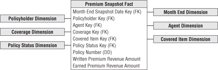
The policyholder, covered item, and coverage dimensions would be identical. The daily date dimension would be replaced with a conformed month dimension table. You don't need to track all the employees who were involved in policy transactions on a monthly basis; it may be useful to retain the involved agent, especially because field operations are so focused on ongoing revenue performance analysis. The transaction type dimension would not be used because it does not apply at the periodic snapshot granularity. Instead, you introduce a status dimension so users can quickly discern the current state of a coverage or policy, such as new policies or cancellations this month and over time.
Conformed Facts
While we're on the topic of conformity, you also need to use conformed facts. If the same facts appear in multiple fact tables, such as facts common to this snapshot fact table as well as the consolidated fact table we'll discuss later in this chapter, then they must have consistent definitions and labels. If the facts are not identical, then they need to be given different names.
Pay-in-Advance Facts
Business management wants to know how much premium revenue was written (or sold) each month, as well as how much revenue was earned. Although a policyholder may contract and pay for coverages on covered items for a period of time, the revenue is not earned until the service is provided. In the case of the insurance company, the revenue from a policy is earned month by month as long as the policyholder doesn't cancel. The correct calculation of a metric like earned premium would mean fully replicating all the business rules of the operational revenue recognition system within the BI application. Typically, the rules for converting a transaction amount into its monthly revenue impact are complex, especially with mid-month coverage upgrades and downgrades. Fortunately, these metrics can be sourced from a separate operational system.
As illustrated in Figure 16.4, we include two premium revenue metrics in the periodic snapshot fact table to handle the different definitions of written versus earned premium. Simplistically, if an annual policy for a given coverage and covered item was written on January 1 for a cost of $600, then the written premium for January would be $600, but the earned premium is $50 ($600 divided by 12 months). In February, the written premium is zero and the earned premium is still $50. If the policy is canceled on March 31, the earned premium for March is $50, while the written premium is a negative $450. Obviously, at this point the earned revenue stream comes to a crashing halt.
Figure 16.4 Periodic premium snapshot schema.
Pay-in-advance business scenarios typically require the combination of transaction and monthly snapshot fact tables to answer questions of transaction frequency and timing, as well as questions of earned income in a given month. You can almost never add enough facts to a snapshot schema to do away with the need for a transaction schema, or vice versa.
Heterogeneous Supertypes and Subtypes Revisited
We are again confronted with the need to look at the snapshot data with more specific line-of-business attributes, and grapple with snapshot facts that vary by line of business. Because the custom facts for each line are incompatible with each other, most of the fact row would be filled with nulls if you include all the line-of-business facts on every row. In this scenario, the answer is to separate the monthly snapshot fact table physically by line of business. You end up with the single supertype monthly snapshot schema and a series of subtype snapshots, one for each line of business or coverage type. Each of the subtype snapshot fact tables is a copy of a segment of the supertype fact table for just those coverage keys and covered item keys belonging to a particular line of business. We include the supertype facts as a convenience so analyses within a coverage type can use both the supertype and custom subtype facts without accessing two large fact tables.
Multivalued Dimensions Revisited
Automobile insurance provides another opportunity to discuss multivalued dimensions. Often multiple insured drivers are associated with a policy. You can construct a bridge table, as illustrated in Figure 16.5, to capture the relationship between the insured drivers and policy. In this case the insurance company can assign realistic weighting factors based on each driver's share of the total premium cost.
Figure 16.5 Bridge table for multiple drivers on a policy.
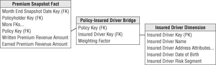
Because these relationships may change over time, you can add effective and expiration dates to the bridge table. Before you know it, you end up with a factless fact table to capture the evolving relationships between a policy, policy holder, covered item, and insured driver over time.
More Insurance Case Study Background
Unfortunately, the insurance business has a downside. We learn from the interviewees that there's more to life than collecting premium revenue payments. The main costs in this industry result from claim losses. After a policy is in effect, then a claim can be made against a specific coverage and covered item. A claimant, who may be the policyholder or a new party not previously known to the insurance company, makes the claim. When the insurance company opens a new claim, a reserve is usually established. The reserve is a preliminary estimate of the insurance company's eventual liability for the claim. As further information becomes known, this reserve can be adjusted.
Before the insurance company pays any claim, there is usually an investigative phase where the insurance company sends out an adjuster to examine the covered item and interview the claimant, policyholder, or other individuals involved. The investigative phase produces a stream of task transactions. In complex claims, various outside experts may be required to pass judgment on the claim and the extent of the damage.
In most cases, after the investigative phase, the insurance company issues a number of payments. Many of these payments go to third parties such as doctors, lawyers, or automotive body shop operators. Some payments may go directly to the claimant. It is important to clearly identify the employee responsible for every payment made against an open claim.
The insurance company may take possession of the covered item after replacing it for the policyholder or claimant. If the item has any remaining value, salvage payments received by the insurance company are a credit against the claim accounting.
Eventually, the payments are completed and the claim is closed. If nothing unusual happens, this is the end of the transaction stream generated by the claim. However, in some cases, further claim payments or claimant lawsuits may force a claim to be reopened. An important measure for an insurance company is how often and under what circumstances claims are reopened.
In addition to analyzing the detailed claims processing transactions, the insurance company also wants to understand what happens over the life of a claim. For example, the time lag between the claim open date and the first payment date is an important measure of claims processing efficiency.
Updated Insurance Bus Matrix
With a better understanding of the claims side of the business, the draft matrix from Figure 16.1 needs to be revisited. Based on the new requirements, you add another row to the matrix to accommodate claim transactions, as shown in Figure 16.6. Many of the dimensions identified earlier in the project will be reused; you add new columns to the matrix for the claim, claimant, and third-party payee.
Figure 16.6 Updated insurance bus matrix.
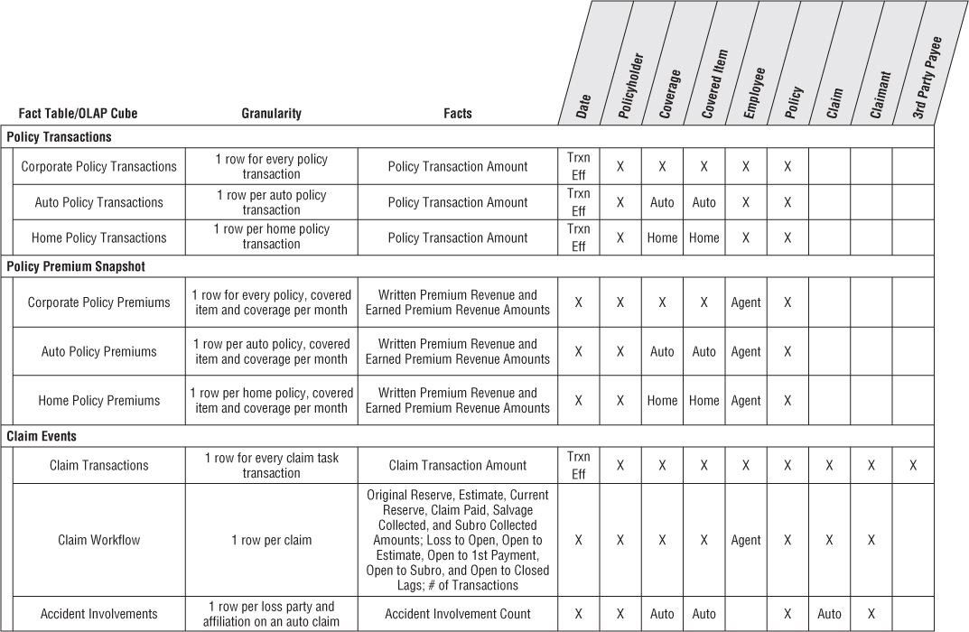
Detailed Implementation Bus Matrix
DW/BI teams sometimes struggle with the level of detail captured in an enterprise data warehouse bus matrix. In the planning phase of an architected DW/BI project, it makes sense to stick with rather high-level business processes (or sources). Multiple fact tables at different levels of granularity may result from each of these business process rows. In the subsequent implementation phase, you can take a subset of the matrix to a lower level of detail by reflecting all the fact tables or OLAP cubes resulting from the process as separate matrix rows. At this point the matrix can be enhanced by adding columns to reflect the granularity and metrics associated with each fact table or cube. Figure 16.7 illustrates a more detailed implementation bus matrix.
Figure 16.7 Detailed implementation bus matrix.
Claim Transactions
The operational claim processing system generates a slew of transactions, including the following transaction task types:
- Open claim, reopen claim, close claim
- Set reserve, reset reserve, close reserve
- Set salvage estimate, receive salvage payment
- Adjuster inspection, adjuster interview
- Open lawsuit, close lawsuit
- Make payment, receive payment
- Subrogate claim
When updating the Figure 16.6 bus matrix, you determine that this schema uses a number of dimensions developed for the policy world. You again have two role-playing dates associated with the claim transactions. Unique column labels should distinguish the claim transaction and effective dates from those associated with policy transactions. The employee is the employee involved in the transactional task. As mentioned in the business case, this is particularly interesting for payment authorization transactions. The claim transaction type dimension would include the transaction types and groupings just listed.
As shown in Figure 16.8 , there are several new dimensions in the claim transaction fact table. The claimant is the party making the claim, typically an individual. The third-party payee may be either an individual or commercial entity. Both the claimant and payee dimensions usually are dirty dimensions because of the difficulty of reliably identifying them across claims. Unscrupulous potential payees may go out of their way not to identify themselves in a way that would easily tie them to other claims in the insurance company's system.
Figure 16.8 Claim transaction schema.

Transaction Versus Profile Junk Dimensions
Beyond the reused dimensions from the policy-centric schemas and the new claim-centric dimensions just listed, there are a large number of indicators and descriptions related to a claim. Designers are sometimes tempted to dump all these descriptive attributes into a claim dimension. This approach makes sense for high-cardinality descriptors, such as the specific address where the loss occurred or a narrative describing the event. However, in general, you should avoid creating dimensions with the same number of rows as the fact table.
As we described in Chapter 6, low-cardinality codified data, like the method used to report the loss or an indicator denoting whether the claim resulted from a catastrophic event, are better handled in a junk dimension. In this case, the junk dimension would more appropriately be referred to as the claim profile dimension with one row per unique combination of profile attributes. Grouping or filtering on the profile attributes would yield faster query responses than if they were alternatively handled as claim dimension attributes.
Claim Accumulating Snapshot
Even with a robust transaction schema, there is a whole class of urgent business questions that can't be answered using only transaction detail. It is difficult to derive claim-to-date performance measures by traversing through every detailed claim task transaction from the beginning of the claim's history and appropriately applying the transactions.
On a periodic basis, perhaps at the close of each day, you can roll forward all the transactions to update an accumulating claim snapshot incrementally. The granularity is one row per claim; the row is created once when the claim is opened and then is updated throughout the life of a claim until it is finally closed.
Many of the dimensions are reusable, conformed dimensions, as illustrated in Figure 16.9. You should include more dates in this fact table to track the key claim milestones and deliver time lags. These lags may be the raw difference between two dates, or they may be calculated in a more sophisticated way by accounting for only workdays in the calculations. A status dimension is added to quickly identify all open, closed, or reopened claims, for example. Transaction-specific dimensions such as employee, payee, and claim transaction type are suppressed, whereas the list of additive, numeric measures has been expanded.
Figure 16.9 Claim accumulating snapshot schema.

Accumulating Snapshot for Complex Workflows
Accumulating snapshot fact tables are typically appropriate for predictable workflows with well-established milestones. They usually have five to 10 key milestone dates representing the pipeline's start, completion, and key events in between. However, sometimes workflows are less predictable. They still have a definite start and end date, but the milestones in between are numerous and less stable. Some occurrences may skip over some intermediate milestones, but there's no reliable pattern.
In this situation, the first task is to identify the key dates that link to role-playing date dimensions. These dates represent the most important milestones. The start and end dates for the process would certainly qualify; in addition, you should consider other commonly occurring critical milestones. These dates (and their associated dimensions) will be used extensively for BI application filtering.
However, if the number of additional milestones is both voluminous and unpredictable, they can't all be handled as additional date foreign keys in the fact table. Typically, business users are more interested in the lags between these milestones, rather than filtering or grouping on the dates themselves. If there were a total of 20 potential milestone events, there would be 190 potential lag durations: event A-to-B, A-to-C, … (19 possible lags from event A), B-to-C, … (18 possible lags from event B), and so on. Instead of physically storing 190 lag metrics, you can get away with just storing 19 of them and then calculate the others. Because every pipeline occurrence starts by passing through milestone A, which is the workflow begin date, you could store all 19 lags from the anchor event A and then calculate the other variations. For example, if you want to know the lag from B-to-C, take the A-to-C lag value and subtract the A-to-B lag. If there happens to be a null for one of the lags involved in a calculation, then the result also needs to be null because one of the events never occurred. But such a null result is handled gracefully if you are counting or averaging that lag across a number of claim rows.
Timespan Accumulating Snapshot
An accumulating snapshot does a great job presenting a workflow's current state, but it obliterates the intermediate states. For example, a claim can move in and out of various states such as opened, denied, closed, disputed, opened again, and closed again. The claim transaction fact table will have separate rows for each of these events, but as discussed earlier, it doesn't accumulate metrics across transactions; trying to re-create the evolution of a workflow from these transactional events would be a nightmare. Meanwhile, a classic accumulating snapshot doesn't allow you to re-create the claim workflow at any arbitrary date in the past.
Alternatively, you could add effective and expiration dates to the accumulating snapshot. In this scenario, instead of destructively updating each row as changes occur, you add a new row that preserves the state of a claim for a span of time. Similar to a type 2 slowly changing dimension, the fact row includes the following additional columns:
- Snapshot start date
- Snapshot end date (updated when a new row for a given claim is added)
- Snapshot current flag (updated when a new row is added)
Most users are only interested in the current view provided by a classic accumulating snapshot; you can meet their needs by defining a view that filters the historical snapshot rows based on the current flag. The minority of users and reports who need to look at the pipeline as of any arbitrary date in the past can do so by filtering on the snapshot start and end dates.
The timespan accumulating snapshot fact table is more complicated to maintain than a standard accumulating snapshot, but the logic is similar. Where the classic accumulating snapshot updates a row, the timespan snapshot updates the administrative columns on the row formerly known as current, and inserts a new row.
Periodic Instead of Accumulating Snapshot
In cases where a claim is not so short-lived, such as with long-term disability or bodily injury claims that have a multiyear life span, you may represent the snapshot as a periodic snapshot rather than an accumulating snapshot. The grain of the periodic snapshot would be one row for every active claim at a regular snapshot interval, such as monthly. The facts would represent numeric, additive facts that occurred during the period such as amount claimed, amount paid, and change in reserve.
Policy/Claim Consolidated Periodic Snapshot
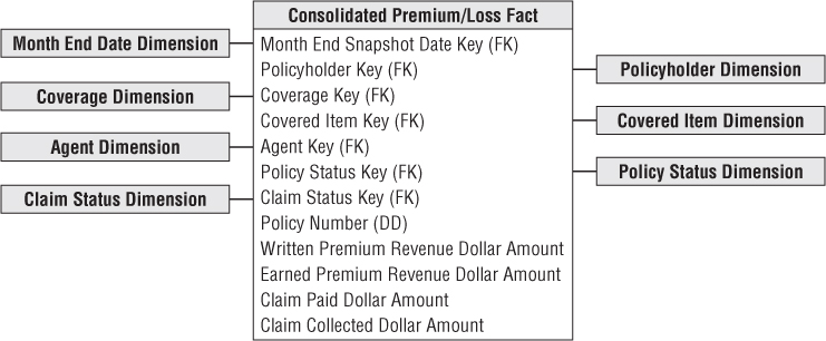
With the fact tables designed thus far, you can deliver a robust perspective of the policy and claim transactions, in addition to snapshots from both processes. However, the business users are also interested in profit metrics. Although premium revenue and claim loss financial metrics could be derived by separately querying two fact tables and then combining the results set, you opt to go the next step in the spirit of ease of use and performance for this common drill-across requirement.
You can construct another fact table that brings together the premium revenue and claim loss metrics, as shown in Figure 16.10. This table has a reduced set of dimensions corresponding to the lowest level of granularity common to both processes. As discussed in Chapter 7: Accounting, this is a consolidated fact table because it combines data from multiple business processes. It is best to develop consolidated fact tables after the base metrics have been delivered in separate atomic dimensional models.
Figure 16.10 Policy/claim consolidated fact table.
Factless Accident Events
We earlier described factless fact tables as the collision of keys at a point in space and time. In the case of an automobile insurer, you can record literal collisions using a factless fact table. In this situation, the fact table registers the many-to-many correlations between the loss parties and loss items, or put in laymen's terms, all the correlations between the people and vehicles involved in an accident.
Two new dimensions appear in the factless fact table shown in Figure 16.11. The loss party captures the individuals involved in the accident, whereas the loss party role identifies them as passengers, witnesses, legal representation, or some other capacity. As we did in Chapter 3: Retail Sales, we include a fact that is always valued at 1 to facilitate counting and aggregation. This factless fact table can represent complex accidents involving many individuals and vehicles because the number of involved parties with various roles is open-ended. When there is more than one claimant or loss party associated with an accident, you can optionally treat these dimensions as multivalued dimensions using claimant group and loss party group bridge tables. This has the advantage that the grain of the fact table is preserved as one record per accident claim. Either schema variation could answer questions such as, “How many bodily injury claims did you handle where ABC Legal Partners represented the claimant and EZ-Dent-B-Gone body shop performed the repair?”
Figure 16.11 Factless fact table for accident involvements.

Common Dimensional Modeling Mistakes to Avoid
As we close this final chapter on dimensional modeling techniques, we thought it would be helpful to establish boundaries beyond which designers should not go. Thus far in this book, we've presented concepts by positively stating dimensional modeling best practices. Now rather than reiterating the to-dos, we focus on not-to-dos by elaborating on dimensional modeling techniques that should be avoided. We've listed the not-to-dos in reverse order of importance; be aware, however, that even the less important mistakes can seriously compromise your DW/BI system.
Mistake 10: Place Text Attributes in a Fact Table
The process of creating a dimensional model is always a kind of triage. The numeric measurements delivered from an operational business process source belong in the fact table. The descriptive textual attributes comprising the context of the measurements go in dimension tables. In nearly every case, if an attribute is used for constraining and grouping, it belongs in a dimension table. Finally, you should make a field-by-field decision about the leftover codes and pseudo-numeric items, placing them in the fact table if they are more like measurements and used in calculations or in a dimension table if they are more like descriptions used for filtering and labeling. Don't lose your nerve and leave true text, especially comment fields, in the fact table. You need to get these text attributes off the main runway of the data warehouse and into dimension tables.
Mistake 9: Limit Verbose Descriptors to Save Space
You might think you are being a conservative designer by keeping the size of the dimensions under control. However, in virtually every data warehouse, the dimension tables are geometrically smaller than the fact tables. Having a 100 MB product dimension table is insignificant if the fact table is one hundred or thousand times as large! Our job as designers of easy-to-use dimensional models is to supply as much verbose descriptive context in each dimension as possible. Make sure every code is augmented with readable descriptive text. Remember the textual attributes in the dimension tables provide the browsing, constraining, or filtering parameters in BI applications, as well as the content for the row and column headers in reports.
Mistake 8: Split Hierarchies into Multiple Dimensions
A hierarchy is a cascaded series of many-to-one relationships. For example, many products roll up to a single brand; many brands roll up to a single category. If a dimension is expressed at the lowest level of granularity, such as product, then all the higher levels of the hierarchy can be expressed as unique values in the product row. Business users understand hierarchies. Your job is to present the hierarchies in the most natural and efficient manner in the eyes of the users, not in the eyes of a data modeler who has focused his entire career on designing third normal form entity-relationship models for transaction processing systems.
A fixed depth hierarchy belongs together in a single physical flat dimension table, unless data volumes or velocity of change dictate otherwise. Resist the urge to snowflake a hierarchy by generating a set of progressively smaller subdimension tables. Finally, if more than one rollup exists simultaneously for a dimension, in most cases it's perfectly reasonable to include multiple hierarchies in the same dimension as long as the dimension has been defined at the lowest possible grain (and the hierarchies are uniquely labeled).
Mistake 7: Ignore the Need to Track Dimension Changes
Contrary to popular belief, business users often want to understand the impact of changes on at least a subset of the dimension tables' attributes. It is unlikely users will settle for dimension tables with attributes that always reflect the current state of the world. Three basic techniques track slowly moving attribute changes; don't rely on type 1 exclusively. Likewise, if a group of attributes changes rapidly, you can split a dimension to capture the more volatile attributes in a mini-dimension.
Mistake 6: Solve All Performance Problems with More Hardware
Aggregates, or derived summary tables, are a cost-effective way to improve query performance. Most BI tool vendors have explicit support for the use of aggregates. Adding expensive hardware should be done as part of a balanced program that includes building aggregates, partitioning, creating indices, choosing query-efficient DBMS software, increasing real memory size, increasing CPU speed, and adding parallelism at the hardware level.
Mistake 5: Use Operational Keys to Join Dimensions and Facts
Novice designers are sometimes too literal minded when designing the dimension tables' primary keys that connect to the fact tables' foreign keys. It is counterproductive to declare a suite of dimension attributes as the dimension table key and then use them all as the basis of the physical join to the fact table. This includes the unfortunate practice of declaring the dimension key to be the operational key, along with an effective date. All types of ugly problems will eventually arise. The dimension's operational or intelligent key should be replaced with a simple integer surrogate key that is sequentially numbered from 1 to N, where N is the total number of rows in the dimension table. The date dimension is the sole exception to this rule.
Mistake 4: Neglect to Declare and Comply with the Fact Grain
All dimensional designs should begin by articulating the business process that generates the numeric performance measurements. Second, the exact granularity of that data must be specified. Building fact tables at the most atomic, granular level will gracefully resist the ad hoc attack. Third, surround these measurements with dimensions that are true to that grain. Staying true to the grain is a crucial step in the design of a dimensional model. A subtle but serious design error is to add helpful facts to a fact table, such as rows that describe totals for an extended timespan or a large geographic area. Although these extra facts are well known at the time of the individual measurement and would seem to make some BI applications simpler, they cause havoc because all the automatic summations across dimensions overcount these higher-level facts, producing incorrect results. Each different measurement grain demands its own fact table.
Mistake 3: Use a Report to Design the Dimensional Model
A dimensional model has nothing to do with an intended report! Rather, it is a model of a measurement process. Numeric measurements form the basis of fact tables. The dimensions appropriate for a given fact table are the context that describes the circumstances of the measurements. A dimensional model is based solidly on the physics of a measurement process and is quite independent of how a user chooses to define a report. A project team once confessed it had built several hundred fact tables to deliver order management data to its business users. It turned out each fact table had been constructed to address a specific report request; the same data was extracted many, many times to populate all these slightly different fact tables. Not surprising, the team was struggling to update the databases within the nightly batch window. Rather than designing a quagmire of report-centric schemas, the team should have focused on the measurement processes. The users' requirements could have been handled with a well-designed schema for the atomic data along with a handful (not hundreds) of performance-enhancing aggregations.
Mistake 2: Expect Users to Query Normalized Atomic Data
The lowest level data is always the most dimensional and should be the foundation of a dimensional design. Data that has been aggregated in any way has been deprived of some of its dimensions. You can't build a dimensional model with aggregated data and expect users and their BI tools to seamlessly drill down to third normal form (3NF) data for the atomic details. Normalized models may be helpful for preparing the data in the ETL kitchen, but they should never be used for presenting the data to business users.
Mistake 1: Fail to Conform Facts and Dimensions
This final not-to-do should be presented as two separate mistakes because they are both so dangerous to a successful DW/BI design, but we've run out of mistake numbers to assign, so they're lumped into one.
It would be a shame to get this far and then build isolated data repository stovepipes. We refer to this as snatching defeat from the jaws of victory. If you have a numeric measured fact, such as revenue, in two or more databases sourced from different underlying systems, then you need to take special care to ensure the technical definitions of these facts exactly match. If the definitions do not exactly match, then they shouldn't both be referred to as revenue. This is conforming the facts.
Finally, the single most important design technique in the dimensional modeling arsenal is conforming dimensions. If two or more fact tables are associated with the same dimension, you must be fanatical about making these dimensions identical or carefully chosen subsets of each other. When you conform dimensions across fact tables, you can drill across separate data sources because the constraints and row headers mean the same thing and match at the data level. Conformed dimensions are the secret sauce needed for building distributed DW/BI environments, adding unexpected new data sources to an existing warehouse, and making multiple incompatible technologies function together harmoniously. Conformed dimensions also allow teams to be more agile because they're not re-creating the wheel repeatedly; this translates into a faster delivery of value to the business community.
Summary
In this final case study we designed a series of insurance dimensional models representing the culmination of many important concepts developed throughout this book. Hopefully, you now feel comfortable and confident using the vocabulary and tools of a dimensional modeler.
With dimensional modeling mastered, in the next chapter we discuss all the other activities that occur during the life of a successful DW/BI project. Before you go forth to be dimensional, it's useful to have this holistic perspective and understanding, even if your job focus is limited to modeling.